Calculate rate of change in oxygen from flowthrough respirometry data
Source:R/calc_rate.ft.R
calc_rate.ft.RdCalculates rate of oxygen uptake or production in flowthrough respirometry
data given a flowrate and delta oxygen values, which can either be directly
entered, or be calculated from inflow and outflow oxygen. The function
returns a single rate value from the whole dataset or a subset of it, by
averaging delta oxygen values. Alternatively, multiple rate values can be
returned from different regions of continuous data, or a rolling rate of a
specific window size performed across the whole dataset.
Usage
calc_rate.ft(
  x = NULL,
  flowrate = NULL,
  from = NULL,
  to = NULL,
  by = NULL,
  width = NULL,
  plot = TRUE,
  ...
)
Arguments
- x
numeric value or vector of delta oxygen values, a 2-column
data.frameof outflow (col 1) and inflow (col 2) oxygen values, or an object of classinspect.ft.- flowrate
numeric value. The flow rate through the respirometer in volume (ul,ml,L) per unit time (s,m,h,d). The units are not necessary here, but will be specified in
convert_rate.ft.- from
numeric value or vector. Defaults to
NULL. The start of the region(s) over which you want to calculate the rate in either time or row units. If a vector, each value must have a paired value into. For use withinspect.ftinputs only.- to
numeric value or vector. Defaults to
NULL. The end of the region(s) over which you want to calculate the rate in either time or row units. If a vector, each value must have a paired value infrom. For use withinspect.ftinputs only.- by
"time"or"row". Defaults to"time". Specifies the units of thefromandby, orwidthvalue. For use withinspect.ftinputs only.- width
numeric. Calculates a rolling rate across the whole dataset of the specified width in the units specified in
by. For use withinspect.ftinputs only.- plot
logical. Defaults to TRUE. Plots the data.
- ...
Allows additional plotting controls to be passed such as
pos,quiet = TRUE,legend = FALSE, andrate.rev = FALSE.
Value
Output is a list object of class calc_rate.ft containing input
parameters and data, various summary data, metadata, and the primary output
of interest $rate, which can be background adjusted in adjust_rate.ft
or converted to units in convert_rate.ft. Note the $summary table
contains linear regression coefficients alongside other metadata. These
should not be confused with those in other functions such as calc_rate
where slopes represent rates and coefficients such as a high r-squared are
important. Here, they represent the stability of the data region, in that
the closer the slope is to zero the less the delta oxygen values, and
therefore rates, in that region vary. These are included to enable possible
future functionality where stable regions may be automatically identified.
Details
calc_rate.ft calculates rates by averaging delta oxygen values across the
whole dataset, or from specified subsets of the data. The flowrate is then
used to convert these average delta values to rates. There are no units
involved in calc_rate.ft. This is a deliberate decision. The units of
oxygen concentration and flowrate will be specified later in
convert_rate.ft() when rates are converted to specific output units.
For continuous data recordings, it is recommended a data.frame containing
the data be prepared via inspect.ft(), and entered as the x input.
For data not prepared like this, x can be a 2-column data.frame
containing numeric values of outflow (col 1) and inflow (col 2) oxygen
concentrations in that order. Alternatively, if x is a numeric value or
vector it is treated as delta oxygen values (outflow oxygen concentration
minus inflow oxygen concentration in the same units). In both these cases,
the from, to, and by inputs are are ignored, and all delta oxygen
values whether as entered or calculated from the inflow and outflow oxygen
columns are converted to rates.
Specifying regions
For calculating rates over specific regions of the data, the from and to
inputs in the by units of "time" (the default) or "row" can be used for
inspect.ft() inputs. All delta oxygen values within this region are
converted to rates, and averaged to produce a overall rate for the region
($rate in the output). Multiple regions can be examined within the same
dataset by entering from and to as vectors of paired values to specify
different regions. In this case, $rate in the output will be a vector of
multiple rates with each result corresponding to the position of the paired
from and to inputs. If from and to are NULL (the default), the rate
is determined over the entire dataset.
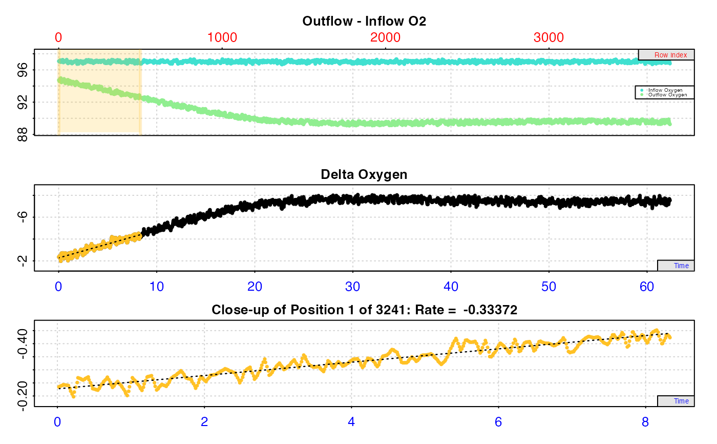
Alternatively a width input can be specified, in which case a rolling rate
is calculated using this window size (in the relevant by units) across the
entire dataset, and returned as a vector of rate values in $rate. See
here
for how this might be used.
Flowrate
In order to convert delta oxygen values to a oxygen uptake or production
rate, the flowrate input is required. This must be in a volume (L, ml, or
ul) per unit time (s,m,h,d), for example in L/s. The units are not required
to be entered here; they will be specified in [convert_rate.ft()] to
convert rates to specific units of oxygen uptake or production.
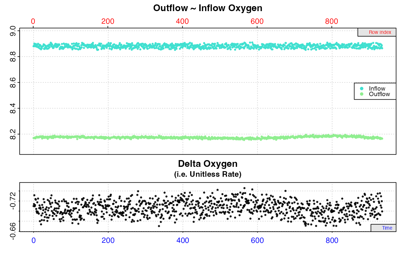
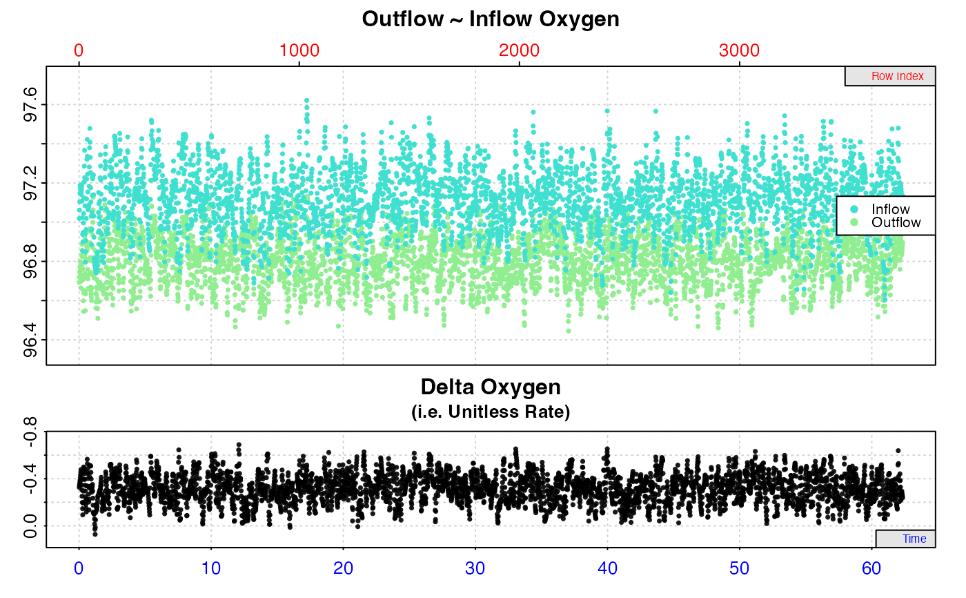
Plot
For rates calculated from inspect.ft inputs, a plot is produced (provided
plot = TRUE) showing the original data timeseries of inflow and outflow
oxygen (if present, top plot), oxygen delta values (middle or top plot) with
the region specified via the from and to inputs highlighted in orange,
and a close-up of this region with calculated rate value (bottom plot). If
multiple rates have been calculated, by default the first is plotted. Others
can be plotted by changing the pos input, e.g. plot(object, pos = 2).
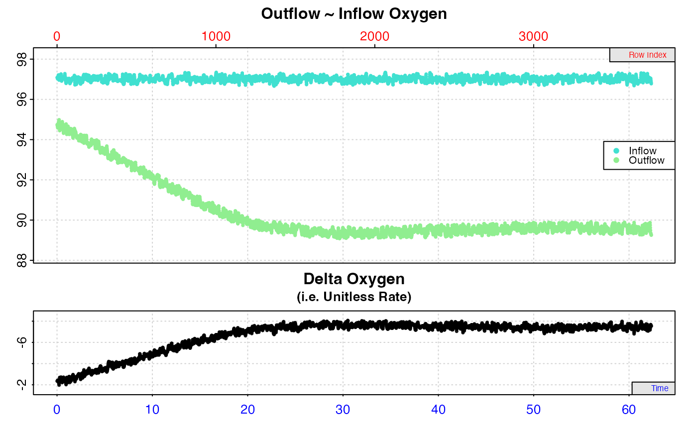
Important: Since respR is primarily used to examine oxygen
consumption, the delta oxygen and rate plots are by default plotted on a
reverse y-axis. In respR oxygen uptake rates are negative since they
represent a negative slope of oxygen against time. In these plots the axis is
reversed so that higher uptake rates (i.e. more negative rates) will be
higher on these plots. If you are interested instead in oxygen production
rates, which are positive, the rate.rev = FALSE input can be passed in
either the inspect.ft call, or when using plot() on the output object. In
this case, the delta and rate values will be plotted numerically, with higher
oxygen production rates higher on the plot.
Additional plotting options
If the legend or labels obscure part of the plot, they can be suppressed via
legend = FALSE in either the inspect.ft call, or when using plot() on
the output object. Console output messages can be suppressed using quiet = TRUE. Console output messages can be suppressed using quiet = TRUE. If
axis labels or other text boxes obscure parts of the plot they can be
suppressed using legend = FALSE. If axis labels (particularly y-axis) are
difficult to read, las = 2 can be passed to make axis labels horizontal,
andoma (outer margins, default oma = c(0.4, 1, 1.5, 0.4)), and mai
(inner margins, default mai = c(0.3, 0.15, 0.35, 0.15)) used to adjust plot
margins.
Background control or "blank" experiments
calc_rate.ft can also be used to determine background rates from empty
control experiments in the same way specimen rates are determined. The saved
objects can be used as the by input in adjust_rate.ft(). For
experiments in which the specimen data is to be corrected by a
concurrently-run control experiment, best option is to use this as the
in.oxy input in inspect.ft(). See help file for that function, or the
vignettes on the website for examples.
S3 Generic Functions
Saved output objects can be used in the generic S3 functions print(),
summary(), and mean().
print(): prints a single result, by default the first rate. Others can be printed by passing theposinput. e.g.print(x, pos = 2)summary(): prints summary table of all results and metadata, or those specified by theposinput. e.g.summary(x, pos = 1:5). The summary can be exported as a separate data frame by passingexport = TRUE.mean(): calculates the mean of all rates, or those specified by theposinput. e.g.mean(x, pos = 1:5)The mean can be exported as a separate value by passingexport = TRUE.
More
For additional help, documentation, vignettes, and more visit the respR
website at https://januarharianto.github.io/respR/
Examples
# Single numeric delta oxygen value. The delta oxygen is the difference
# between inflow and outflow oxygen.
calc_rate.ft(-0.8, flowrate = 1.6)
#> calc_rate.ft: Calculating rate from delta oxygen value(s).
#> calc_rate.ft: Plot only available for 'inspect.ft' inputs.
#>
#> # print.calc_rate.ft # ------------------
#> Rank 1 of 1 rates:
#> Rate: -1.28
#>
#> To see full results use summary().
#> -----------------------------------------
# Numeric vector of multiple delta oxygen values
ft_rates <- calc_rate.ft(c(-0.8, -0.88, -0.9, -0.76), flowrate = 1.6)
#> calc_rate.ft: Calculating rate from delta oxygen value(s).
#> calc_rate.ft: Plot only available for 'inspect.ft' inputs.
print(ft_rates)
#>
#> # print.calc_rate.ft # ------------------
#> Rank 1 of 4 rates:
#> Rate: -1.28
#>
#> To see other results use 'pos' input.
#> To see full results use summary().
#> -----------------------------------------
summary(ft_rates)
#>
#> # summary.calc_rate.ft # ----------------
#> Summary of all rate results:
#>
#> rep rank intercept_b0 slope_b1 rsq row endrow time endtime oxy endoxy delta_mean flowrate rate
#> 1: NA 1 NA NA NA NA NA NA NA NA NA -0.80 1.6 -1.280
#> 2: NA 2 NA NA NA NA NA NA NA NA NA -0.88 1.6 -1.408
#> 3: NA 3 NA NA NA NA NA NA NA NA NA -0.90 1.6 -1.440
#> 4: NA 4 NA NA NA NA NA NA NA NA NA -0.76 1.6 -1.216
#> -----------------------------------------
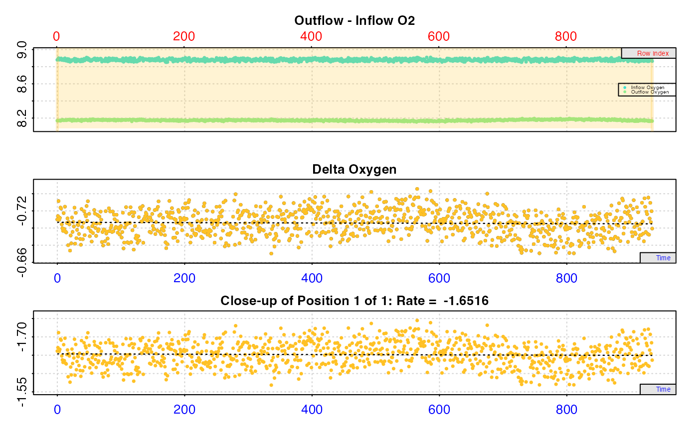
# Calculate rate from entire dataset
inspect.ft(flowthrough.rd, time = 1, out.oxy = 2, in.oxy = 3, ) %>%
calc_rate.ft(flowrate = 2.34)
#> inspect.ft: No issues detected while inspecting data frame.
#>
#> # print.inspect.ft # --------------------
#> time oxy.out oxy.in
#> numeric pass pass pass
#> Inf/-Inf pass pass pass
#> NA/NaN pass pass pass
#> sequential pass - -
#> duplicated pass - -
#> evenly-spaced pass - -
#>
#> -----------------------------------------
 #> calc_rate.ft: Calculating rate from 'inspect.ft' object.
#> calc_rate.ft: 'from' and 'to' inputs NULL. Applying default of calculating rate from entire dataset.
#> calc_rate.ft: Calculating rate from 'inspect.ft' object.
#> calc_rate.ft: 'from' and 'to' inputs NULL. Applying default of calculating rate from entire dataset.
 #>
#> # print.calc_rate.ft # ------------------
#> Rank 1 of 1 rates:
#> Rate: -1.651558
#>
#> To see full results use summary().
#> -----------------------------------------
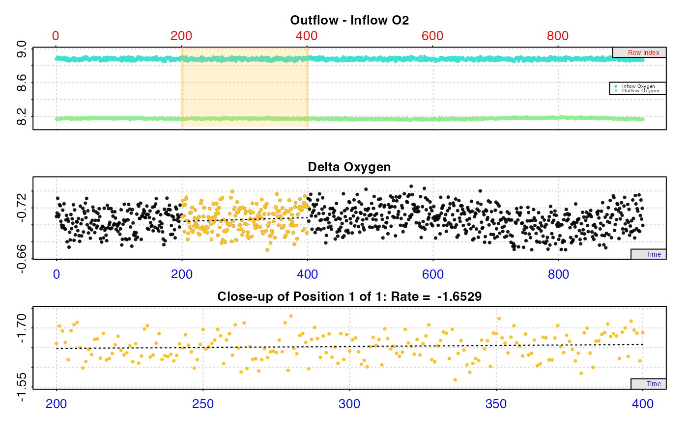
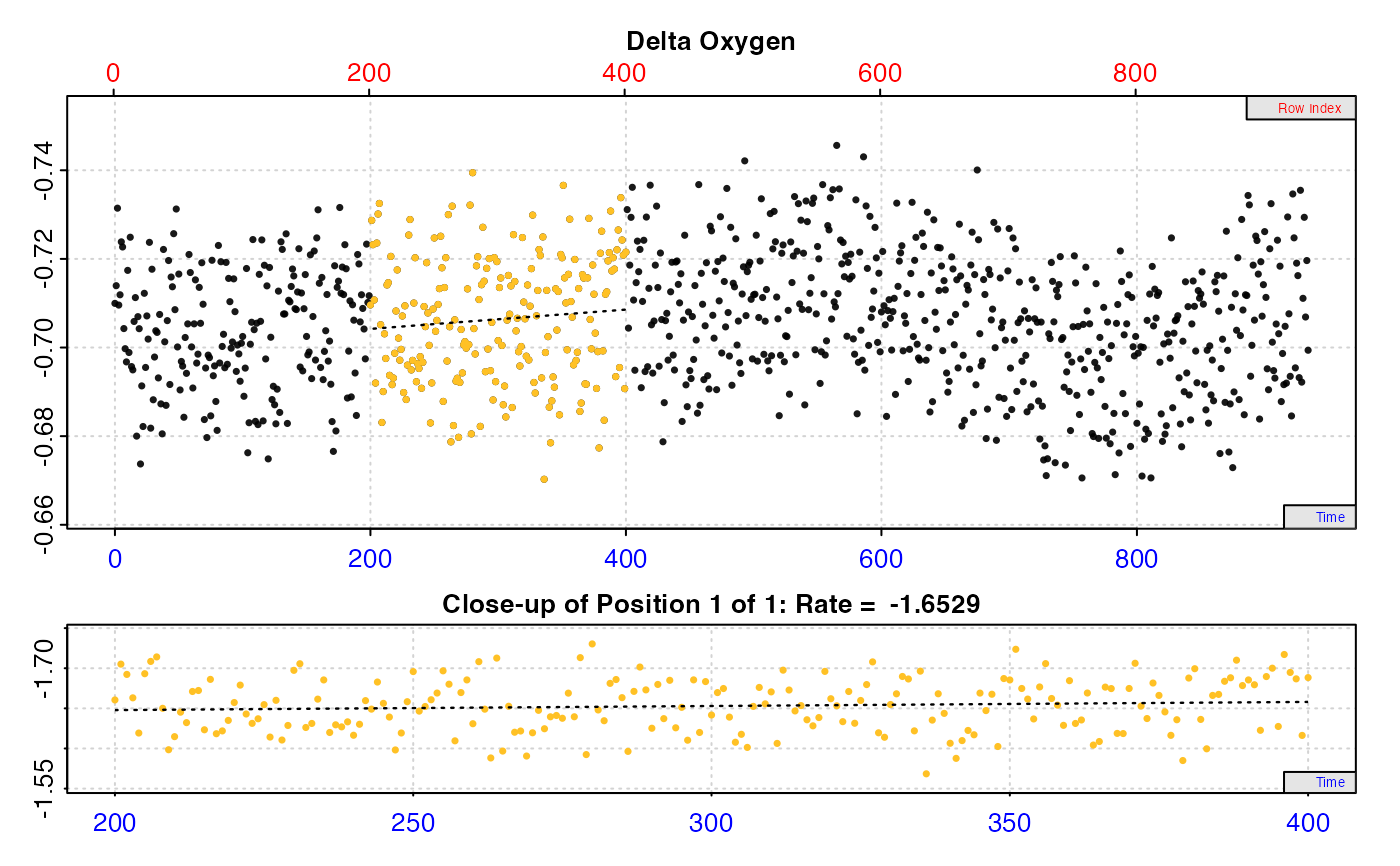
# Calculate rate from a region based on time
inspect.ft(flowthrough.rd, time = 1, out.oxy = 2, in.oxy = 3, ) %>%
calc_rate.ft(flowrate = 2.34, from = 200, to = 400, by = "time")
#> inspect.ft: No issues detected while inspecting data frame.
#>
#> # print.inspect.ft # --------------------
#> time oxy.out oxy.in
#> numeric pass pass pass
#> Inf/-Inf pass pass pass
#> NA/NaN pass pass pass
#> sequential pass - -
#> duplicated pass - -
#> evenly-spaced pass - -
#>
#> -----------------------------------------
#>
#> # print.calc_rate.ft # ------------------
#> Rank 1 of 1 rates:
#> Rate: -1.651558
#>
#> To see full results use summary().
#> -----------------------------------------
# Calculate rate from a region based on time
inspect.ft(flowthrough.rd, time = 1, out.oxy = 2, in.oxy = 3, ) %>%
calc_rate.ft(flowrate = 2.34, from = 200, to = 400, by = "time")
#> inspect.ft: No issues detected while inspecting data frame.
#>
#> # print.inspect.ft # --------------------
#> time oxy.out oxy.in
#> numeric pass pass pass
#> Inf/-Inf pass pass pass
#> NA/NaN pass pass pass
#> sequential pass - -
#> duplicated pass - -
#> evenly-spaced pass - -
#>
#> -----------------------------------------
 #> calc_rate.ft: Calculating rate from 'inspect.ft' object.
 #>
#> # print.calc_rate.ft # ------------------
#> Rank 1 of 1 rates:
#> Rate: -1.652933
#>
#> To see full results use summary().
#> -----------------------------------------
# Calculate rate from multiple regions
inspect.ft(flowthrough.rd, time = 1, out.oxy = 2, in.oxy = 3, ) %>%
calc_rate.ft(flowrate = 2.34,
from = c(200, 400, 600),
to = c(300, 500, 700),
by = "row") %>%
summary()
#> inspect.ft: No issues detected while inspecting data frame.
#>
#> # print.inspect.ft # --------------------
#> time oxy.out oxy.in
#> numeric pass pass pass
#> Inf/-Inf pass pass pass
#> NA/NaN pass pass pass
#> sequential pass - -
#> duplicated pass - -
#> evenly-spaced pass - -
#>
#> -----------------------------------------
#>
#> # print.calc_rate.ft # ------------------
#> Rank 1 of 1 rates:
#> Rate: -1.652933
#>
#> To see full results use summary().
#> -----------------------------------------
# Calculate rate from multiple regions
inspect.ft(flowthrough.rd, time = 1, out.oxy = 2, in.oxy = 3, ) %>%
calc_rate.ft(flowrate = 2.34,
from = c(200, 400, 600),
to = c(300, 500, 700),
by = "row") %>%
summary()
#> inspect.ft: No issues detected while inspecting data frame.
#>
#> # print.inspect.ft # --------------------
#> time oxy.out oxy.in
#> numeric pass pass pass
#> Inf/-Inf pass pass pass
#> NA/NaN pass pass pass
#> sequential pass - -
#> duplicated pass - -
#> evenly-spaced pass - -
#>
#> -----------------------------------------
 #> calc_rate.ft: Calculating rate from 'inspect.ft' object.
 #>
#> # summary.calc_rate.ft # ----------------
#> Summary of all rate results:
#>
#> rep rank intercept_b0 slope_b1 rsq row endrow time endtime oxy endoxy delta_mean flowrate rate
#> 1: NA 1 -0.7092250 0.00001420935 0.0008778610 200 300 199 299 -0.7116950 -0.7193922 -0.7056869 2.34 -1.651307
#> 2: NA 2 -0.7143960 0.00001099438 0.0005300532 400 500 399 499 -0.6907237 -0.6974397 -0.7094595 2.34 -1.660135
#> 3: NA 3 -0.7441011 0.00005622227 0.0146175225 600 700 599 699 -0.6990357 -0.7172883 -0.7076128 2.34 -1.655814
#> -----------------------------------------
# Calculate rate from existing delta oxygen values
inspect.ft(flowthrough.rd, time = 1, delta.oxy = 4) %>%
calc_rate.ft(flowrate = 2.34, from = 200, to = 400, by = "time")
#> inspect.ft: No issues detected while inspecting data frame.
#>
#> # print.inspect.ft # --------------------
#> time oxy.delta
#> numeric pass pass
#> Inf/-Inf pass pass
#> NA/NaN pass pass
#> sequential pass -
#> duplicated pass -
#> evenly-spaced pass -
#>
#> -----------------------------------------
#>
#> # summary.calc_rate.ft # ----------------
#> Summary of all rate results:
#>
#> rep rank intercept_b0 slope_b1 rsq row endrow time endtime oxy endoxy delta_mean flowrate rate
#> 1: NA 1 -0.7092250 0.00001420935 0.0008778610 200 300 199 299 -0.7116950 -0.7193922 -0.7056869 2.34 -1.651307
#> 2: NA 2 -0.7143960 0.00001099438 0.0005300532 400 500 399 499 -0.6907237 -0.6974397 -0.7094595 2.34 -1.660135
#> 3: NA 3 -0.7441011 0.00005622227 0.0146175225 600 700 599 699 -0.6990357 -0.7172883 -0.7076128 2.34 -1.655814
#> -----------------------------------------
# Calculate rate from existing delta oxygen values
inspect.ft(flowthrough.rd, time = 1, delta.oxy = 4) %>%
calc_rate.ft(flowrate = 2.34, from = 200, to = 400, by = "time")
#> inspect.ft: No issues detected while inspecting data frame.
#>
#> # print.inspect.ft # --------------------
#> time oxy.delta
#> numeric pass pass
#> Inf/-Inf pass pass
#> NA/NaN pass pass
#> sequential pass -
#> duplicated pass -
#> evenly-spaced pass -
#>
#> -----------------------------------------
 #> calc_rate.ft: Calculating rate from 'inspect.ft' object.
 #>
#> # print.calc_rate.ft # ------------------
#> Rank 1 of 1 rates:
#> Rate: -1.652933
#>
#> To see full results use summary().
#> -----------------------------------------
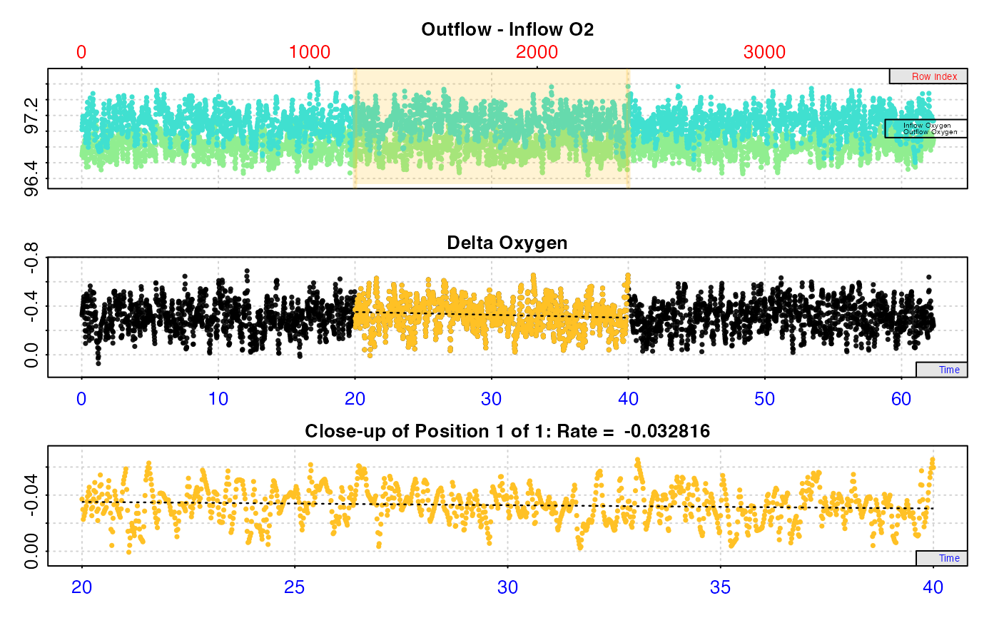
# Calculate rate from a background recording
inspect.ft(flowthrough_mult.rd,
time = 1,
out.oxy = 5,
in.oxy = 9) %>%
calc_rate.ft(flowrate = 0.1, from = 20, to = 40, by = "time") %>%
summary()
#> Warning: inspect.ft: Time values are not evenly-spaced (numerically).
#> inspect.ft: Data issues detected. For more information use print().
#>
#> # print.inspect.ft # --------------------
#> num.time oxy.out.blank oxy.in.blank
#> numeric pass pass pass
#> Inf/-Inf pass pass pass
#> NA/NaN pass pass pass
#> sequential pass - -
#> duplicated pass - -
#> evenly-spaced WARN - -
#>
#> Uneven Time data locations (first 20 shown) in column: num.time
#> [1] 1 2 3 4 5 6 7 8 9 10 11 12 13 14 15 16 17 18 19 20
#> Minimum and Maximum intervals in uneven Time data:
#> [1] 0.01 0.02
#> -----------------------------------------
#>
#> # print.calc_rate.ft # ------------------
#> Rank 1 of 1 rates:
#> Rate: -1.652933
#>
#> To see full results use summary().
#> -----------------------------------------
# Calculate rate from a background recording
inspect.ft(flowthrough_mult.rd,
time = 1,
out.oxy = 5,
in.oxy = 9) %>%
calc_rate.ft(flowrate = 0.1, from = 20, to = 40, by = "time") %>%
summary()
#> Warning: inspect.ft: Time values are not evenly-spaced (numerically).
#> inspect.ft: Data issues detected. For more information use print().
#>
#> # print.inspect.ft # --------------------
#> num.time oxy.out.blank oxy.in.blank
#> numeric pass pass pass
#> Inf/-Inf pass pass pass
#> NA/NaN pass pass pass
#> sequential pass - -
#> duplicated pass - -
#> evenly-spaced WARN - -
#>
#> Uneven Time data locations (first 20 shown) in column: num.time
#> [1] 1 2 3 4 5 6 7 8 9 10 11 12 13 14 15 16 17 18 19 20
#> Minimum and Maximum intervals in uneven Time data:
#> [1] 0.01 0.02
#> -----------------------------------------
 #> calc_rate.ft: Calculating rate from 'inspect.ft' object.
 #>
#> # summary.calc_rate.ft # ----------------
#> Summary of all rate results:
#>
#> rep rank intercept_b0 slope_b1 rsq row endrow time endtime oxy endoxy delta_mean flowrate rate
#> 1: NA 1 -0.3988676 0.002357015 0.01261235 1200 2400 20 40 -0.3708712 -0.5964118 -0.3281571 0.1 -0.03281571
#> -----------------------------------------
# Calculate a rolling rate
inspect.ft(flowthrough_mult.rd,
time = 1,
out.oxy = 2,
in.oxy = 6) %>%
calc_rate.ft(flowrate = 0.1, width = 500, by = "row") %>%
summary()
#> Warning: inspect.ft: Time values are not evenly-spaced (numerically).
#> inspect.ft: Data issues detected. For more information use print().
#>
#> # print.inspect.ft # --------------------
#> num.time oxy.out.1 oxy.in.1
#> numeric pass pass pass
#> Inf/-Inf pass pass pass
#> NA/NaN pass pass pass
#> sequential pass - -
#> duplicated pass - -
#> evenly-spaced WARN - -
#>
#> Uneven Time data locations (first 20 shown) in column: num.time
#> [1] 1 2 3 4 5 6 7 8 9 10 11 12 13 14 15 16 17 18 19 20
#> Minimum and Maximum intervals in uneven Time data:
#> [1] 0.01 0.02
#> -----------------------------------------
#>
#> # summary.calc_rate.ft # ----------------
#> Summary of all rate results:
#>
#> rep rank intercept_b0 slope_b1 rsq row endrow time endtime oxy endoxy delta_mean flowrate rate
#> 1: NA 1 -0.3988676 0.002357015 0.01261235 1200 2400 20 40 -0.3708712 -0.5964118 -0.3281571 0.1 -0.03281571
#> -----------------------------------------
# Calculate a rolling rate
inspect.ft(flowthrough_mult.rd,
time = 1,
out.oxy = 2,
in.oxy = 6) %>%
calc_rate.ft(flowrate = 0.1, width = 500, by = "row") %>%
summary()
#> Warning: inspect.ft: Time values are not evenly-spaced (numerically).
#> inspect.ft: Data issues detected. For more information use print().
#>
#> # print.inspect.ft # --------------------
#> num.time oxy.out.1 oxy.in.1
#> numeric pass pass pass
#> Inf/-Inf pass pass pass
#> NA/NaN pass pass pass
#> sequential pass - -
#> duplicated pass - -
#> evenly-spaced WARN - -
#>
#> Uneven Time data locations (first 20 shown) in column: num.time
#> [1] 1 2 3 4 5 6 7 8 9 10 11 12 13 14 15 16 17 18 19 20
#> Minimum and Maximum intervals in uneven Time data:
#> [1] 0.01 0.02
#> -----------------------------------------
 #> calc_rate.ft: Calculating rate from 'inspect.ft' object.
#> calc_rate.ft: Rates determined using a rolling 'width' of 500 row values.
#> calc_rate.ft: Calculating rate from 'inspect.ft' object.
#> calc_rate.ft: Rates determined using a rolling 'width' of 500 row values.
 #>
#> # summary.calc_rate.ft # ----------------
#> Summary of all rate results:
#>
#> rep rank intercept_b0 slope_b1 rsq row endrow time endtime oxy endoxy delta_mean flowrate rate
#> 1: NA 1 -2.273550 -0.254777842 0.9185171054 1 500 0.02 8.33 -2.343996 -4.233047 -3.337248 0.1 -0.3337248
#> 2: NA 2 -2.273909 -0.254556409 0.9181911883 2 501 0.03 8.35 -2.365692 -4.181305 -3.340923 0.1 -0.3340923
#> 3: NA 3 -2.274182 -0.254339605 0.9178474112 3 502 0.05 8.37 -2.387388 -4.169322 -3.344530 0.1 -0.3344530
#> 4: NA 4 -2.274270 -0.254166479 0.9175696569 4 503 0.07 8.38 -2.409084 -4.184013 -3.348123 0.1 -0.3348123
#> 5: NA 5 -2.274182 -0.254032586 0.9173537179 5 504 0.08 8.40 -2.430780 -4.198703 -3.351702 0.1 -0.3351702
#> ---
#> 3237: NA 3237 -7.340111 -0.001702673 0.0004962938 3237 3736 53.95 62.27 -7.429813 -7.679898 -7.439051 0.1 -0.7439051
#> 3238: NA 3238 -7.324342 -0.001980779 0.0006700266 3238 3737 53.97 62.28 -7.243068 -7.641992 -7.439475 0.1 -0.7439475
#> 3239: NA 3239 -7.327742 -0.001934161 0.0006393082 3239 3738 53.98 62.30 -7.056323 -7.604086 -7.440197 0.1 -0.7440197
#> 3240: NA 3240 -7.350430 -0.001561031 0.0004197082 3240 3739 54.00 62.32 -6.996323 -7.566180 -7.441217 0.1 -0.7441217
#> 3241: NA 3241 -7.381539 -0.001044124 0.0001899277 3241 3740 54.02 62.33 -7.125256 -7.528274 -7.442281 0.1 -0.7442281
#> -----------------------------------------
#>
#> # summary.calc_rate.ft # ----------------
#> Summary of all rate results:
#>
#> rep rank intercept_b0 slope_b1 rsq row endrow time endtime oxy endoxy delta_mean flowrate rate
#> 1: NA 1 -2.273550 -0.254777842 0.9185171054 1 500 0.02 8.33 -2.343996 -4.233047 -3.337248 0.1 -0.3337248
#> 2: NA 2 -2.273909 -0.254556409 0.9181911883 2 501 0.03 8.35 -2.365692 -4.181305 -3.340923 0.1 -0.3340923
#> 3: NA 3 -2.274182 -0.254339605 0.9178474112 3 502 0.05 8.37 -2.387388 -4.169322 -3.344530 0.1 -0.3344530
#> 4: NA 4 -2.274270 -0.254166479 0.9175696569 4 503 0.07 8.38 -2.409084 -4.184013 -3.348123 0.1 -0.3348123
#> 5: NA 5 -2.274182 -0.254032586 0.9173537179 5 504 0.08 8.40 -2.430780 -4.198703 -3.351702 0.1 -0.3351702
#> ---
#> 3237: NA 3237 -7.340111 -0.001702673 0.0004962938 3237 3736 53.95 62.27 -7.429813 -7.679898 -7.439051 0.1 -0.7439051
#> 3238: NA 3238 -7.324342 -0.001980779 0.0006700266 3238 3737 53.97 62.28 -7.243068 -7.641992 -7.439475 0.1 -0.7439475
#> 3239: NA 3239 -7.327742 -0.001934161 0.0006393082 3239 3738 53.98 62.30 -7.056323 -7.604086 -7.440197 0.1 -0.7440197
#> 3240: NA 3240 -7.350430 -0.001561031 0.0004197082 3240 3739 54.00 62.32 -6.996323 -7.566180 -7.441217 0.1 -0.7441217
#> 3241: NA 3241 -7.381539 -0.001044124 0.0001899277 3241 3740 54.02 62.33 -7.125256 -7.528274 -7.442281 0.1 -0.7442281
#> -----------------------------------------