Intermittent-flow respirometry: Long experiment
Source:vignettes/intermittent_long.Rmd
intermittent_long.RmdThis vignette shows a intermittent-flow analysis from a lengthy experiment, with over 100 replicates and a background rate that changes over the course of the experiment. This type of experiment is one many fish physiologists in particular will be familiar with.
The example data (zeb_intermittent.rd) was kindly
provided by Dr. Davide
Thambithurai, and is from an experiment on a zebrafish. It is
comprised of one replicate of 14 minutes duration (12 minutes recording,
2 minutes flushing), followed by 105 replicates of 11 minutes duration
(9 minutes recording, 2 minutes flushing). In addition there are pre-
and post-experiment background recordings. See
help(zeb_intermittent.rd) for row locations of all
stages.
See vignette("intermittent_short") for an example with a
smaller dataset, which covers in more detail the basics of analysing
intermittent-flow data and is a better starting point if you are new to
respR or analysing these types of experiment. Even if not,
we would recommend reading both before starting your analysis.
Experiment overview
From this experiment dataset we want to extract several metrics:
Pre- and post-experiment background rates. Background rates were recorded at the start and end of the experiment (initial and end sections with shallow slopes). This was a lengthy experiment in high temperatures, and so the microbial background rate increases substantially over the course of the experiment. We will assume this increase is constant (i.e. linear), and each replicate rate will be adjusted with a background rate calculated according its time within the experiment. That is, later replicates will be adjusted by a greater amount.
Maximum metabolic rate (MMR). Before this experiment the fish had been exercised to exhaustion, then immediately placed in the respirometer. The first replicate during which it is recovering from the accrued oxygen debt will represent MMR.
Routine metabolic rate (RMR). This will be calculated using the later replicates once the animal has recovered from the exercise. This is generally defined as the routine use of oxygen to fuel basal metabolism and minor spontaneous movements for maintaining station or posture.
Standard metabolic rate (SMR). Sometimes also known as basal or minimum metabolic rate. This is also calculated using the later replicates once the animal has recovered. This is generally defined as the lowest oxygen use rates observed, which are representative of the requirements of basal metabolism only.
Which of these last two metrics is valid or appropriate to report depends on the organism and the circumstances and aims of the experiments. Their definitions are widely debated, and there is a huge literature on the differences between these physiological metrics. See here for some papers discussing these. Here, we will show how to extract what may be regarded as both RMR and SMR from this dataset.
Analysis methods
Extracting the background rates and MMR are relatively straightforward and will be covered in their own sections.
After this, we will show two different approaches to extract RMR and
SMR using respR functions. The first
uses the dedicated calc_rate.int() function to run
calc_rate on each replicate to extract a rate from the same
data region of each, before filtering these to get the RMR. The second uses the dedicated auto_rate.int()
function to run auto_rate on each replicate to extract the
lowest rate from each of a specified width, before filtering these to
get the SMR.
Please note: You should not simply copy and
repeat the following code on your own data. They are examples to show
how the respR functions are adaptable and flexible and how
rates can be extracted, filtered and selected to arrive at a final
reportable rate in a variety of ways. They are not recommendations that
you should use these specific approaches for particular outputs. There
is a massive
literature around respirometry, the different physiological metrics,
and how to quantify them. Before analysis of your own data you should
familiarise yourself with it, with similar experiments in the
literature, and the current state of best practices in the field. Many
factors such as appropriate regions or widths to extract rates from,
method used to extract rates, and final selection criteria differ
between experiments for very good reasons, in that every study is
different. It is important to select appropriate analysis factors
objectively and report them in your methods. See especially Killen
et al. (2021) and Prinzing
et al. (2021).
Note we use the native pipe operator (|>) introduced
in R
v4.1 for much of the following. These can be substituted for
dpylr pipes (%>%) if you have not yet
updated, or alternatively save output objects and enter them into the
next function.
Inspecting the data
inspect() is the general respR function for
visualising and inspecting data prior to analysis, and saving it to an
object that can be used in subsequent functions. This is a very large
dataset (nearly 80,000 rows), so if running the code in this vignette
note that operations may take some time.
Before progressing, we’ll inspect a portion of the data at the start without saving the result to show the structure.
zeb_intermittent.rd |>
  subset_data(from = 1, to = 18000, by = "row") |>
  inspect()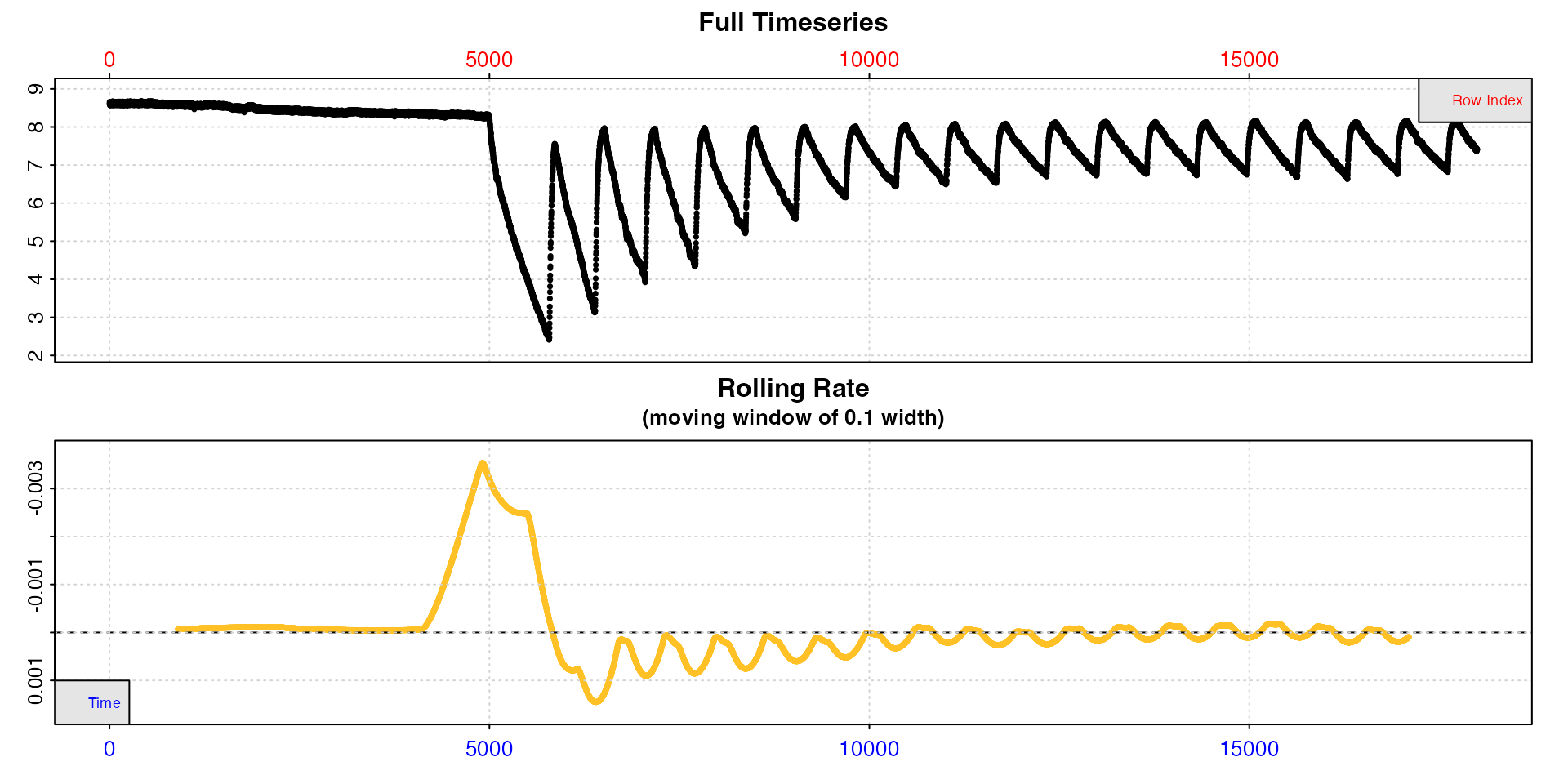
The top plot shows the initial background recording up to row 5000, the first replicate of 14 minutes duration to determine MMR, followed by replicates of 11 minutes duration. We can see in these oxygen decreasing, separated by regular flushes where it increases back to ambient levels. The bottom plot, a rolling rate across a window of 10% of the data, is not particularly useful as this window will include multiple replicates.
We can similarly have a quick look at the end of the dataset.
zeb_intermittent.rd |>
  subset_data(from = 65000, by = "row") |>
  inspect(width = 0.01)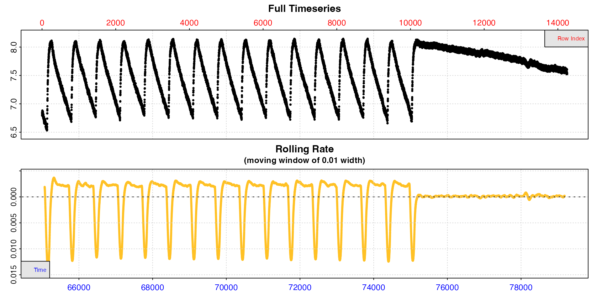
We can see that by the end of the experiment the replicates are much
more regular, suggesting rates have stabilised, and we can also see the
end background recording. This time we passed a different
width to inspect, so the rolling rate plot is
across a 1% window. This makes it slightly more useful, and we can see
within each replicate rates seem to be consistent at around -0.0025,
while the background rate is much lower and closer to zero (dashed
line).
Now that we are fairly satisfied the experiment looks as expected we can inspect the entire dataset and this time save the result to an object we will use for the rest of the analysis.
zeb <- inspect(zeb_intermittent.rd)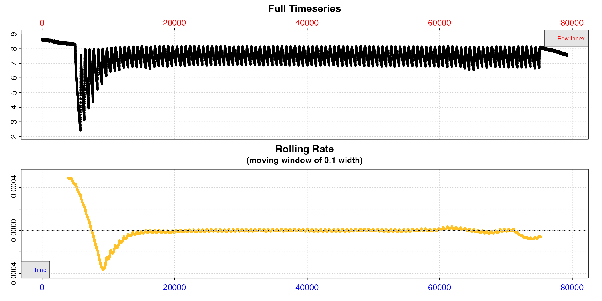
Here because the dataset is so large the plots are of limited use, but we can at least see that much more oxygen was used in the early replicates, as would be expected because the specimen was exercised prior to the experiment, after which they stabilise and are more regular.
Background rates
The initial and end sections of the data will be used to calculate
background rates and how they change over the course of the experiment.
Timepoints of these will typically have been recorded as part of the
experiment, so can be used to subset the relevant sections (see
?zeb_intermittent.rd for row locations of all stages).
We subset these regions from the inspect object we just
saved above, and save them as separate calc_rate.bg
objects.
bg_pre <- zeb |>
  subset_data(from = 1, to = 4999, by = "row") |>
  calc_rate.bg()

bg_post <- zeb |>
  subset_data(from = 75140, to = 79251, by = "row") |>
  calc_rate.bg()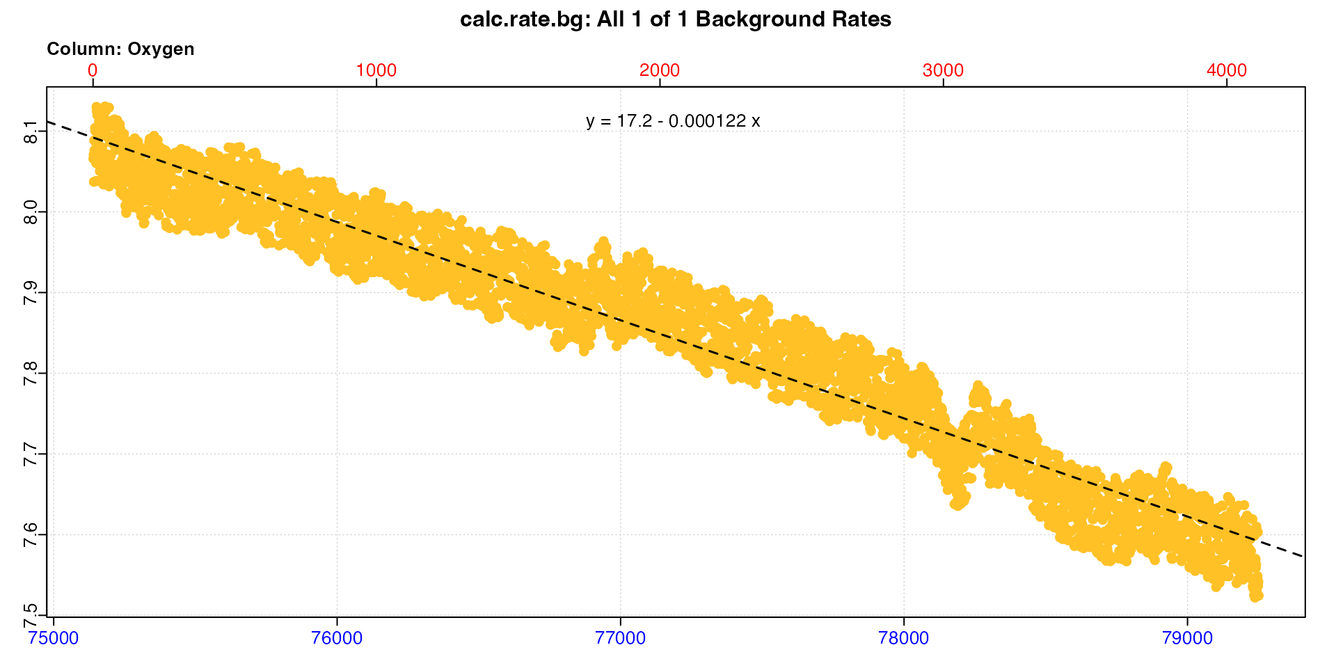
The two different background rates (only the post-experiment plot is shown above) have been saved to these two objects. We can see the actual values by printing them:
bg_pre
#>
#> # print.calc_rate.bg # ------------------
#> Background rate(s):
#> [1] -0.0000742
#> Mean background rate:
#> [1] -0.0000742
#> -----------------------------------------
bg_post
#>
#> # print.calc_rate.bg # ------------------
#> Background rate(s):
#> [1] -0.0001217
#> Mean background rate:
#> [1] -0.0001217
#> -----------------------------------------
We can see the background rate increases by around 70% over the course of the experiment. We will use these later to apply a dynamic background adjustment to specimen rates based on their time during the experiment.
MMR
Here we calculate maximum metabolic rate (MMR) from the first replicate. This replicate is longer than the others; 14 mins (840 rows) vs. 11 mins (660 rows) for all others.
Subset
Here, we subset the first replicate which starts at row 5000 and is
14 minutes long (840 rows) to a separate inspect object,
excluding the two minutes of flush (120 rows) at the end, and plot it to
see how the rate changes over the replicate.
# subset rep 1
zeb_rep_1 <- subset_data(zeb,
                         from = 5000,
                         to = 5000 + 840 - 120,
                         by = "row") |>
  plot(width = 0.2)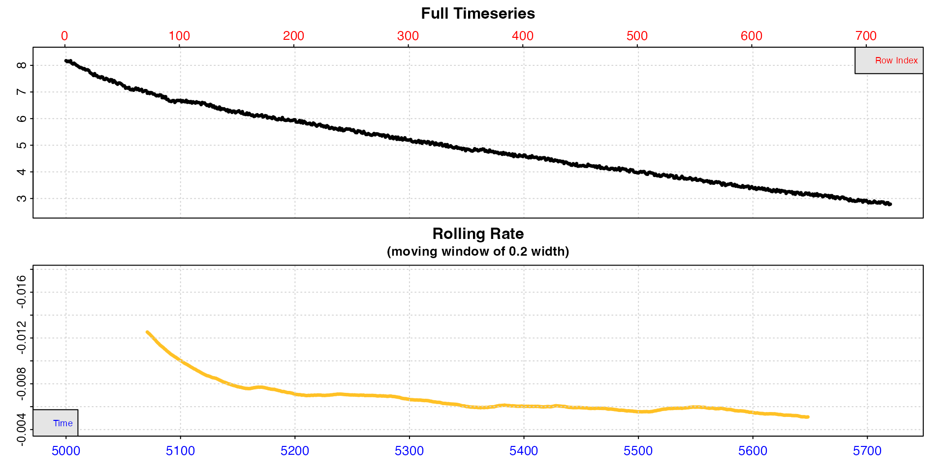
In this replicate, the rolling rate plot shows that calculated at
this particular width, the rate declines rapidly from
around -0.012 to around -0.008, then declines more slowly over the
course of the replicate (note we pass a higher width than
the default 0.1 to smooth the rolling rate a little more). This is as we
would expect from an animal recovering from exercise. However the very
initial stages of replicates are often unstable and excluded from rate
analysis (usually known as the “wait” phase). Therefore we will probably
want to extract our MMR rate after this initial stage but before it
declines too much.
Extract rates
We will show three different ways of extracting what could be defined
as an MMR. First, we will use calc_rate() to extract a rate
from a single specific region. Secondly, we will use the
auto_rate "highest" method to automatically
extract the highest rate of a specific width. Lastly, we will use the
auto_rate "linear" method with the default
inputs to identify linear regions of the data and choose the highest
from amongst these. In this last example we will also show how to adjust
and convert rates, then filter them using select_rate() to
arrive at a final reportable result.
1. calc_rate
This function (see vignette("calc_rate")) simply allows
you to extract a rate (or multiple rates) from a specified row, time, or
oxygen region. In the later example for extracting
rates from the other replicates using calc_rate.int() we
use the same three minute wait phase and five minute
measure phase in each replicate. We will use the same here
to allow for comparison with those rates. This is fairly common practice
in respirometry studies and perfectly acceptable, in that it is
objective and consistent.
zeb_mmr <- calc_rate(zeb_rep_1,
                     from = 180, # three minutes 'wait' after start
                     to = 480,   # five minutes later = 'measure' phase
                     by = "row") |>
  summary()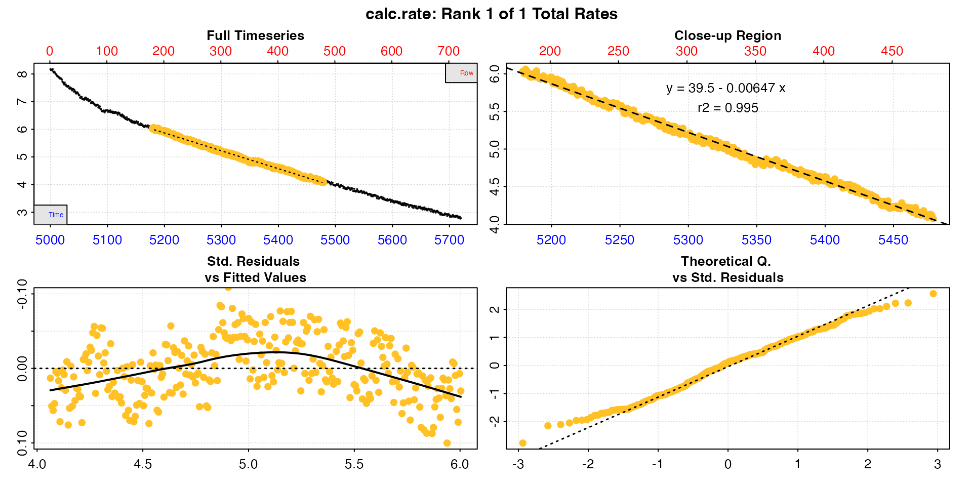
#>
#> # summary.calc_rate # -------------------
#> Summary of all rate results:
#>
#>    rep rank intercept_b0 slope_b1   rsq row endrow time endtime  oxy endoxy rate.2pt     rate
#> 1:  NA    1         39.5 -0.00647 0.995 180    480 5179    5479 6.03   4.08 -0.00653 -0.00647
#> -----------------------------------------
We can see the rate as the final column in summary, and this would be perfectly acceptable to report as the MMR as long as the analysis criteria were also included. See option 3 for how to adjust and convert the rate.
2. auto_rate method = "highest"
auto_rate also allows you to also extract rates of a
specific time or row width, but in contrast to calc_rate it
calculates every rate of this width across the dataset and then
orders them in various ways. One method is to order by highest absolute
value to get the highest uptake rate.
Here we run this method and choose a width of two
minutes (120 rows), that is the function will calculate every rate of
this width and order them from highest to lowest. We use the same three
minute wait phase to exclude the initial part of the
replicate, and for that we use subset_data() to remove the
first 180 rows, then pipe the output to auto_rate (we could
also have done this when we first subset and inspected the data above).
zeb_mmr <- zeb_rep_1 |>
  subset_data(from = 180, by = "row") |>
  auto_rate(method = "highest",
            width = 120,
            by = "row") |>
  summary()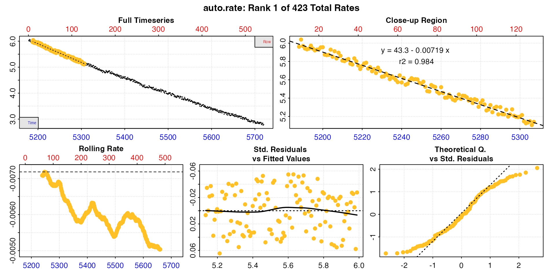
#>
#> # summary.auto_rate # -------------------
#>
#> === Summary of Results by Highest Rate ===
#>      rep rank intercept_b0 slope_b1   rsq density row endrow time endtime  oxy endoxy     rate
#>   1:  NA    1         43.3 -0.00719 0.984      NA  10    129 5188    5307 5.96   5.14 -0.00719
#>   2:  NA    2         43.2 -0.00718 0.984      NA   9    128 5187    5306 5.98   5.11 -0.00718
#>   3:  NA    3         43.2 -0.00718 0.984      NA  11    130 5189    5308 6.04   5.17 -0.00718
#>   4:  NA    4         43.2 -0.00717 0.984      NA  14    133 5192    5311 5.93   5.07 -0.00717
#>   5:  NA    5         43.2 -0.00717 0.984      NA  15    134 5193    5312 5.94   5.14 -0.00717
#>  ---
#> 419:  NA  419         31.7 -0.00505 0.971      NA 420    539 5598    5717 3.41   2.84 -0.00505
#> 420:  NA  420         31.7 -0.00505 0.971      NA 419    538 5597    5716 3.37   2.79 -0.00505
#> 421:  NA  421         31.6 -0.00503 0.971      NA 423    542 5601    5720 3.37   2.79 -0.00503
#> 422:  NA  422         31.6 -0.00503 0.971      NA 421    540 5599    5718 3.44   2.84 -0.00503
#> 423:  NA  423         31.6 -0.00503 0.971      NA 422    541 5600    5719 3.39   2.77 -0.00503
#>
#> Regressions : 423 | Results : 423 | Method : highest | Roll width : 120 | Roll type : row
#> -----------------------------------------
We have already seen that rates are high at the start and then decline across the replicate, so it’s not a surprise that the highest rates are from early in the replicate. We can see our MMR under these criteria would be the first row of this summary table. See next section for how these multiple rates can be adjusted, converted, and filtered to get a final output rate.
3. auto_rate method = "linear"
Here we simply run auto_rate and let the default inputs
be applied to find the linear regions of the data. Be sure to read
help("auto_rate") and vignette("auto_rate") to
understand what this method does, appropriate inputs and how to modify
the defaults. We again subset the data to remove the initial 3
minutes.
zeb_mmr <- zeb_rep_1 |>
  subset_data(from = 180, by = "row") |>
  auto_rate() |>
  summary()
#>
#> # summary.auto_rate # -------------------
#>
#> === Summary of Results by Kernel Density Rank ===
#>    rep rank intercept_b0 slope_b1   rsq density row endrow time endtime  oxy endoxy     rate
#> 1:  NA    1         36.3 -0.00588 0.996    1199 122    450 5300    5628 5.20   3.27 -0.00588
#> 2:  NA    2         32.0 -0.00511 0.981     644 394    541 5572    5719 3.56   2.77 -0.00511
#> 3:  NA    3         37.6 -0.00612 0.991     425 102    304 5280    5482 5.35   4.10 -0.00612
#> 4:  NA    4         37.6 -0.00612 0.991     420 101    304 5279    5482 5.31   4.10 -0.00612
#> 5:  NA    5         42.9 -0.00711 0.979     417   4    111 5182    5289 6.04   5.22 -0.00711
#> 6:  NA    6         41.1 -0.00678 0.985     412  52    184 5230    5362 5.63   4.84 -0.00678
#> 7:  NA    7         36.7 -0.00595 0.986     405 305    451 5483    5629 4.15   3.19 -0.00595
#>
#> Regressions : 435 | Results : 7 | Method : linear | Roll width : 108 | Roll type : row
#> -----------------------------------------
The function has found seven linear regions. All of these rates are
valid results depending on the question being asked, in that they have
been found to be linear regions, and so of consistently sustained rates.
In this case, since we are interested in the maximum rate, the fifth
ranked result has the highest rate value, and comes from
early in the replicate, so is probably the result we are most interested
in. We can plot it using pos.
plot(zeb_mmr, pos = 5)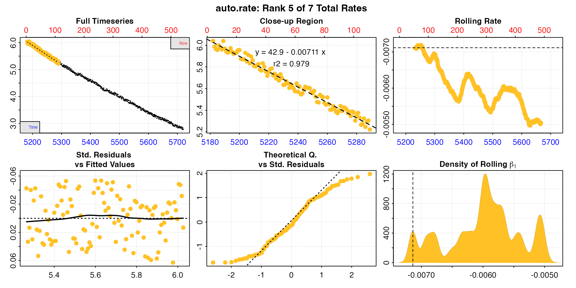
Many aspects will feed into rate selection criteria for a specific experiment or study, and it depends on these whether this in an acceptable, reportable result. Maybe at less than 2 minutes this is not a long enough duration for us to be comfortable that this was a sustained MMR. In which case perhaps one of the other results is better reported. Or maybe we could report an average of some of the rates, such as the top three. The important thing is to apply these selection criteria consistently and report them alongside results.
Changing the width
These are all valid options, as long as they are reported. However,
we can also change the analysis parameters. The width input
in auto_rate determines the width of the rolling
regressions used to find linear regions. See auto_rate()
and other vignettes for full details, but briefly in the case of the
"linear" method this is the starting point for the
analysis. Resulting regressions will vary in width, but in general the
minimum width will be increased by increasing the width.
The default value is 0.2, representing 20% of the data length. Here,
with 10 minutes of data this would represent 2 minutes, which is quite a
brief time window. So instead we will increase this to 0.5 (it can also
be specified in the units of the "by" input).
See Prinzing et al. (2021) for an excellent discussion of appropriate widths in rolling regressions to determine MMR.
zeb_mmr <- zeb_rep_1 |>
  subset_data(from = 180, by = "row") |>
  auto_rate(width = 0.5) |>
  summary()
#>
#> # summary.auto_rate # -------------------
#>
#> === Summary of Results by Kernel Density Rank ===
#>    rep rank intercept_b0 slope_b1   rsq density row endrow time endtime  oxy endoxy     rate
#> 1:  NA    1         36.2 -0.00586 0.996    4258 146    447 5324    5625 5.03   3.30 -0.00586
#> 2:  NA    2         34.6 -0.00556 0.993    1231 260    517 5438    5695 4.33   2.93 -0.00556
#> 3:  NA    3         36.6 -0.00592 0.993     963 119    363 5297    5541 5.21   3.75 -0.00592
#> 4:  NA    4         34.6 -0.00557 0.993     900 259    514 5437    5692 4.36   2.96 -0.00557
#> 5:  NA    5         39.3 -0.00642 0.994     738  31    277 5209    5455 5.86   4.21 -0.00642
#> 6:  NA    6         38.5 -0.00629 0.993     731  55    296 5233    5474 5.65   4.10 -0.00629
#>
#> Regressions : 272 | Results : 6 | Method : linear | Roll width : 271 | Roll type : row
#> -----------------------------------------
Now we have six results varying between 4 and 5 minutes duration, and they are much more consistent in rate value. In this case the fifth result has the highest rate, is early in the replicate, and so is likely a good estimation of MMR. Note how the rolling rate plot is smoother with this higher width.
plot(zeb_mmr, pos = 5)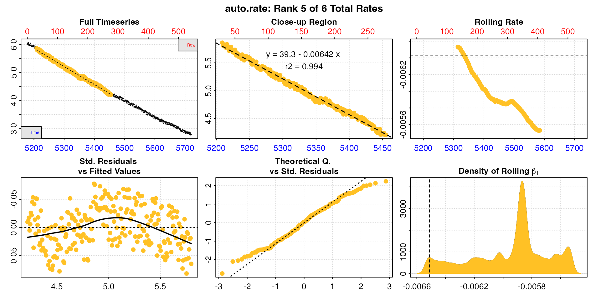
With non-linear data like this, such as from an animal recovering from exercise, increasing the width over which a rate is determined will necessarily decrease the rate values. The researcher needs to keep this in mind, and find a balance between a width that provides a good estimation of the specimen’s physiological state, but also is not affected by other factors such as data noise or anomalies. Most importantly, these decisions and criteria should be reported.
High width values can lead to overfitting and mis-estimation of
rates, and low widths underfitting and rate values which are too
sensitive to data noise. See here
for discussion of this in the context of auto_rate, and how
to choose an appropriate width. We recommend reading Prinzing
et al. (2021) to understand the nuances of determining MMR and
regression widths. See also Killen
et al. (2021).
Adjust
The adjust_rate() function allows rates to be background
adjusted in a number of ways. See vignette("adjust_rate")
for examples. Here we will use it to apply a dynamic linear correction
using the start and end background rates we determined earlier. Essentially this calculates the
appropriate background adjustment for a rate using the time at which it
was determined, assuming the background rate increases linearly from the
pre- to post-experiment values.
For MMR, we will adjust the results from option 3 above, but this
will work with the other options also. We have our saved
auto_rate object, so it’s relatively easy to adjust. We
just need to enter the two background rate objects we saved earlier and
specify the method.
zeb_mmr_adj <- adjust_rate(zeb_mmr,
                           by = bg_pre,     # first background rate
                           by2 = bg_post,   # second background rate
                           method = "linear")
#> adjust_rate: Rate adjustments applied using "linear" method.
summary(zeb_mmr_adj)
#>
#> # summary.adjust_rate # -----------------
#>
#> Adjustment was applied using 'linear' method.
#> Summary of all rate results:
#>
#>    rep rank intercept_b0 slope_b1   rsq density row endrow time endtime  oxy endoxy     rate adjustment rate.adjusted
#> 1:  NA    1         36.2 -0.00586 0.996    4258 146    447 5324    5625 5.03   3.30 -0.00586 -0.0000761      -0.00578
#> 2:  NA    2         34.6 -0.00556 0.993    1231 260    517 5438    5695 4.33   2.93 -0.00556 -0.0000761      -0.00549
#> 3:  NA    3         36.6 -0.00592 0.993     963 119    363 5297    5541 5.21   3.75 -0.00592 -0.0000760      -0.00585
#> 4:  NA    4         34.6 -0.00557 0.993     900 259    514 5437    5692 4.36   2.96 -0.00557 -0.0000761      -0.00550
#> 5:  NA    5         39.3 -0.00642 0.994     738  31    277 5209    5455 5.86   4.21 -0.00642 -0.0000760      -0.00635
#> 6:  NA    6         38.5 -0.00629 0.993     731  55    296 5233    5474 5.65   4.10 -0.00629 -0.0000760      -0.00622
#> -----------------------------------------
There are several things to note here. We can see the ultimate
adjustment value is small in comparison to the rate of the
specimen, as it should be in most experiments. Also, the adjustment
values differ slightly; they are lower for rates that come from the
start of the replicate. This is what we would expect because we are
assuming the background rate is increasing over time.
adjust_rate uses the midpoint time of each rate regression
to calculate the appropriate adjustment value, so earlier rates will
have a lower background adjustment. Lastly, the adjustments are very
close in value to the pre-experiment background rate of
-0.0000742 we established earlier. Again, this is what we would expect
because this is the first replicate and conducted just after the first
background recording. If we are assuming there is a linear increase in
background rate over time this would mean they should be very close in
value.
See later section for how adjustment values differ in other replicates.
Convert
Now that the rates have been adjusted we can convert them to units. This will convert every rate in the object.
The convert_rate function can output rates as
absolute, that is of the whole animal or chamber,
mass-specific if a mass is entered, or
area-specific if an area is entered. The
output.unit should be correctly formatted for whichever of
these are chosen, that is in the order Oxygen/Time, Oxygen/Time/Mass, or
Oxygen/Time/Area.
Note the volume input is volume of water in the
respirometer, not the volume of the respirometer. That is, it
represents the effective volume. A specimen will displace some
of the water, therefore this is the volume of the respirometer minus the
volume of the specimen. There are several approaches to calculate the
effective volume or specimen volume: geometrically; through displacement
in a separate vessel; or calculated from the mass and density. For
example, fish are often assumed to have an equal density as water (~1000
kg/m^3), so their mass is measured, converted to volume and subtracted
from the respirometer volume. Volume could also be determined directly
by pouring out and measuring the water at the end of the experiment, or
by weighing the respirometer. See the respfun
respirometry utilities package for functions to calculate the effective
volume and convert water mass to volume.
Here we use the adjust_rate object saved in the previous
step, and we’ll convert to a mass-specific rate.
zeb_mmr_adj_conv <- convert_rate(zeb_mmr_adj,
                                 oxy.unit = "mg/L",       # oxygen units of the original raw data
                                 time.unit = "secs",      # time units of the original raw data
                                 output.unit = "mg/h/g",  # desired output unit
                                 volume = 0.12,           # effective volume of the respirometer in L
                                 mass = 0.0009)           # mass of the specimen in kg

summary(zeb_mmr_adj_conv)
#>
#> # summary.convert_rate # ----------------
#> Summary of all converted rates:
#>
#>    rep rank intercept_b0 slope_b1   rsq density row endrow time endtime  oxy endoxy     rate adjustment rate.adjusted rate.input oxy.unit time.unit volume   mass area  S  t  P rate.abs rate.m.spec rate.a.spec output.unit rate.output
#> 1:  NA    1         36.2 -0.00586 0.996    4258 146    447 5324    5625 5.03   3.30 -0.00586 -0.0000761      -0.00578   -0.00578     mg/L       sec   0.12 0.0009   NA NA NA NA    -2.50       -2.78          NA   mgO2/hr/g       -2.78
#> 2:  NA    2         34.6 -0.00556 0.993    1231 260    517 5438    5695 4.33   2.93 -0.00556 -0.0000761      -0.00549   -0.00549     mg/L       sec   0.12 0.0009   NA NA NA NA    -2.37       -2.63          NA   mgO2/hr/g       -2.63
#> 3:  NA    3         36.6 -0.00592 0.993     963 119    363 5297    5541 5.21   3.75 -0.00592 -0.0000760      -0.00585   -0.00585     mg/L       sec   0.12 0.0009   NA NA NA NA    -2.53       -2.81          NA   mgO2/hr/g       -2.81
#> 4:  NA    4         34.6 -0.00557 0.993     900 259    514 5437    5692 4.36   2.96 -0.00557 -0.0000761      -0.00550   -0.00550     mg/L       sec   0.12 0.0009   NA NA NA NA    -2.37       -2.64          NA   mgO2/hr/g       -2.64
#> 5:  NA    5         39.3 -0.00642 0.994     738  31    277 5209    5455 5.86   4.21 -0.00642 -0.0000760      -0.00635   -0.00635     mg/L       sec   0.12 0.0009   NA NA NA NA    -2.74       -3.05          NA   mgO2/hr/g       -3.05
#> 6:  NA    6         38.5 -0.00629 0.993     731  55    296 5233    5474 5.65   4.10 -0.00629 -0.0000760      -0.00622   -0.00622     mg/L       sec   0.12 0.0009   NA NA NA NA    -2.69       -2.98          NA   mgO2/hr/g       -2.98
#> -----------------------------------------
The $summary table contains all rate regression
parameters and data locations, adjustments (if applied), units, and
more. In fact it contains all relevant information about the
analysis and is a great way of saving the results, especially using the
export = TRUE input to save it as a data frame. One handy
tip: you may want to enter S, t, and
P even if they are not required for conversions to the
output rate unit because they are saved in the $summary
table, and this can help in keeping track of results across different
experiments. Note the row and endrow columns
will refer to rows of the most recent subset of the data, however the
time and endtime will always refer back to the
time values of original raw data.
Select
The last analysis step is to select our final reportable MMR from the
multiple rates we determined using the linear method. We
saw earlier that after changing some analysis
parameters one of the MMR rates, the 5th in the summary table, was
higher than the others.
summary(zeb_mmr_adj_conv)
#>
#> # summary.convert_rate # ----------------
#> Summary of all converted rates:
#>
#>    rep rank intercept_b0 slope_b1   rsq density row endrow time endtime  oxy endoxy     rate adjustment rate.adjusted rate.input oxy.unit time.unit volume   mass area  S  t  P rate.abs rate.m.spec rate.a.spec output.unit rate.output
#> 1:  NA    1         36.2 -0.00586 0.996    4258 146    447 5324    5625 5.03   3.30 -0.00586 -0.0000761      -0.00578   -0.00578     mg/L       sec   0.12 0.0009   NA NA NA NA    -2.50       -2.78          NA   mgO2/hr/g       -2.78
#> 2:  NA    2         34.6 -0.00556 0.993    1231 260    517 5438    5695 4.33   2.93 -0.00556 -0.0000761      -0.00549   -0.00549     mg/L       sec   0.12 0.0009   NA NA NA NA    -2.37       -2.63          NA   mgO2/hr/g       -2.63
#> 3:  NA    3         36.6 -0.00592 0.993     963 119    363 5297    5541 5.21   3.75 -0.00592 -0.0000760      -0.00585   -0.00585     mg/L       sec   0.12 0.0009   NA NA NA NA    -2.53       -2.81          NA   mgO2/hr/g       -2.81
#> 4:  NA    4         34.6 -0.00557 0.993     900 259    514 5437    5692 4.36   2.96 -0.00557 -0.0000761      -0.00550   -0.00550     mg/L       sec   0.12 0.0009   NA NA NA NA    -2.37       -2.64          NA   mgO2/hr/g       -2.64
#> 5:  NA    5         39.3 -0.00642 0.994     738  31    277 5209    5455 5.86   4.21 -0.00642 -0.0000760      -0.00635   -0.00635     mg/L       sec   0.12 0.0009   NA NA NA NA    -2.74       -3.05          NA   mgO2/hr/g       -3.05
#> 6:  NA    6         38.5 -0.00629 0.993     731  55    296 5233    5474 5.65   4.10 -0.00629 -0.0000760      -0.00622   -0.00622     mg/L       sec   0.12 0.0009   NA NA NA NA    -2.69       -2.98          NA   mgO2/hr/g       -2.98
#> -----------------------------------------
In this case, we could fairly confidently report this as our MMR of
-3.05 mg/h/g. However, the select_rate() function allows
you to filter rates by applying selection criteria. This example will
select and extract the highest n rates to a new object, in
this case the highest single rate. This is quite a simplistic example,
but see later and vignette("select_rate") for more advanced
examples including how to apply multiple criteria.
MMR <- select_rate(zeb_mmr_adj_conv,
                   method = "highest",
                   n = 1)
#> select_rate: Selecting highest 1 *absolute* rate values...
#> ----- Selection complete. 5 rate(s) removed, 1 rate(s) remaining -----
If we need to save any of the other regression data for this rate,
summary has additional inputs that are useful:
pos allows specific rows of summary tables to be extracted,
and export allows it to be saved as a separate data frame.
Here, we’ll use this on the final object to export the coefficients and
other data for this rate.
mmr_results <- summary(MMR, export = TRUE)
mmr_results
#>      rep  rank intercept_b0 slope_b1   rsq density   row endrow  time endtime   oxy endoxy     rate adjustment rate.adjusted rate.input oxy.unit time.unit volume   mass   area      S      t      P rate.abs rate.m.spec rate.a.spec output.unit rate.output
#>    <num> <int>        <num>    <num> <num>   <num> <int>  <int> <num>   <num> <num>  <num>    <num>      <num>         <num>      <num>   <char>    <char>  <num>  <num> <lgcl> <lgcl> <lgcl> <lgcl>    <num>       <num>      <lgcl>      <char>       <num>
#> 1:    NA     5         39.3 -0.00642 0.994     738    31    277  5209    5455  5.86   4.21 -0.00642  -0.000076      -0.00635   -0.00635     mg/L       sec   0.12 0.0009     NA     NA     NA     NA    -2.74       -3.05          NA   mgO2/hr/g       -3.05
Complete MMR analysis
This is the complete analysis we have just conducted to get MMR.
mmr_results <-
  zeb_rep_1 |>                              # using the inspected replicate 1 data...
  subset_data(from = 180,
              by = "row") |>                # subset to apply a 'wait' period
  auto_rate(width = 0.5) |>                 # use auto_rate to get most linear regions
  adjust_rate(by = bg_pre,
              by2 = bg_post,
              method = "linear") |>         # adjust
  convert_rate(oxy.unit = "mg/L",
               time.unit = "secs",
               output.unit = "mg/h/g",
               volume = 0.12,
               mass = 0.0009) |>            # convert
  select_rate(method = "highest",
              n = 1) |>                     # select highest rate
  summary(export = TRUE)                    # final reportable result
#> rep rank intercept_b0 slope_b1 rsq density row endrow time endtime oxy endoxy rate adjustment rate.adjusted rate.input oxy.unit time.unit volume mass area S t P rate.abs rate.m.spec rate.a.spec output.unit rate.output
#> <num> <int> <num> <num> <num> <num> <int> <int> <num> <num> <num> <num> <num> <num> <num> <num> <char> <char> <num> <num> <lgcl> <lgcl> <lgcl> <lgcl> <num> <num> <lgcl> <char> <num>
#> 1: NA 5 39.3 -0.00642 0.994 738 31 277 5209 5455 5.86 4.21 -0.00642 -0.000076 -0.00635 -0.00635 mg/L sec 0.12 0.0009 NA NA NA NA -2.74 -3.05 NA mgO2/hr/g -3.05This allows you to document all analysis parameters and rate selection criteria so that they can be consistently applied and reported alongside the results. See Reporting section for how analyses might be reported concisely in text.
RMR
calc_rate.int
To extract a rate from every replicate and calculate a routine
metabolic rate (RMR) from amongst the results we will use
calc_rate.int(). To repeat the note from above, this is not a recommendation that this is
how you should extract an RMR from your own data; it is simply an
example of one approach and how the respR functions are
flexible and adaptable. calc_rate.int was introduced in respR v2.1
and allows you to specify a replicate structure and run
calc_rate on each replicate to extract a rate from the same
time or row region in each. See vignette("calc_rate.int")
for details of the functionality.
The difference between this and the approach below using auto_rate.int() is that you
specify a region over which to calculate a rate, and this will be the
same in each replicate. This takes away some of the objectivity in
determining rates that auto_rate allows for, but as long as
selection criteria are reported and applied consistently is a perfectly
valid way of processing intermittent-flow data.
We’ve shown above how to get background rates and MMR, so we will use
calc_rate.int to extract a rate from the same region of
each replicate and filter these rates to report an RMR. In these data,
after the first replicate of 14 minutes duration for MMR there is a regular structure of 105 replicates of 11
minutes duration including the flush.
Subset data
In the examples here
we had to specify the start and end location of every replicate in
calc_rate.int. However, if replicates cycle at a regular
interval we can simply enter this as starts. This tells the
function that starting from row 1 replicates cycle at this regular
interval, and it can be entered as a row interval or a duration in time,
as specified using the by input. We only need to subset the
data so that the first replicate starts at row 1 before passing it to
calc_rate.int.
We start by subsetting the data so that the 105 regularly-spaced
replicates start at row 1, that is we exclude the starting background
recording, the first replicate for MMR, and the end background
recording. We then inspect it.
zeb_insp <- zeb_intermittent.rd |>
  subset_data(from = 5840,
              to = 75139,
              by = "row") |>
  inspect()
#> inspect: Applying column default of 'time = 1'
#> inspect: Applying column default of 'oxygen = 2'
#> inspect: No issues detected while inspecting data frame.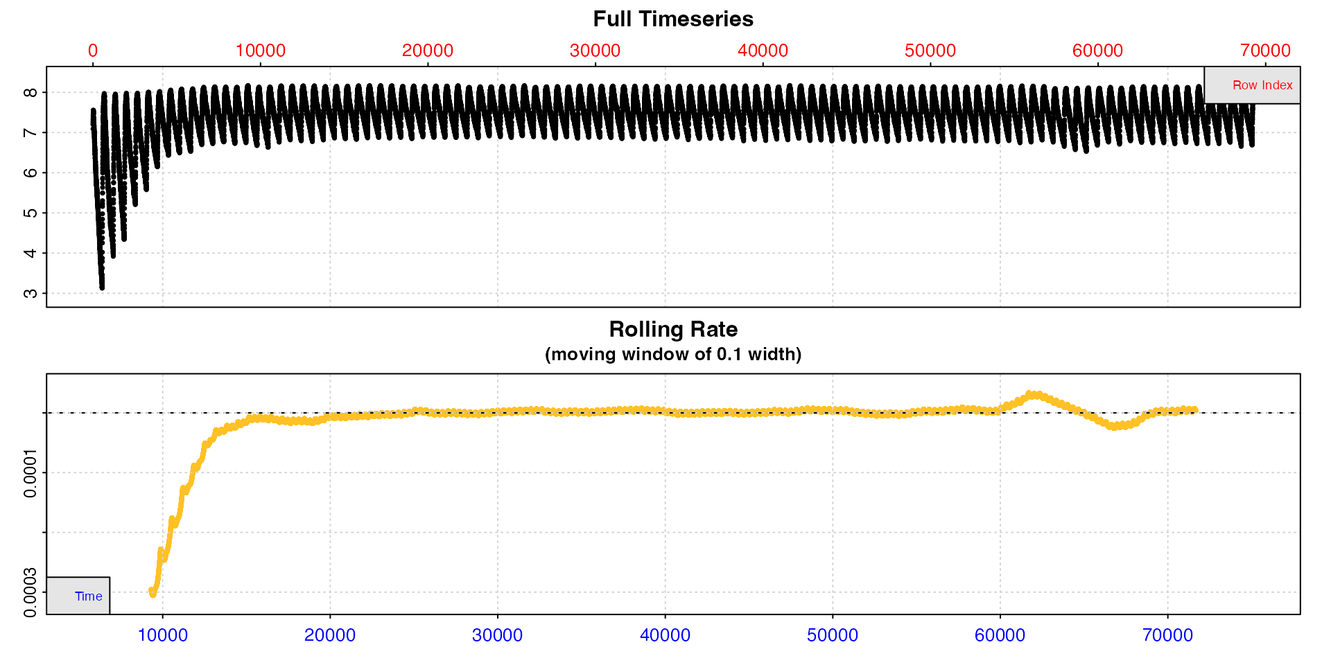
Extract rates
Now we run calc_rate.int and specify a 660 row interval
between replicates using starts. We’ll calculate a rate
across the same five minute time period in each replicate, from three
minutes to eight minutes. To do this we specify a 180 row
wait phase and 300 row measure phase.
zeb_cr.int <- calc_rate.int(zeb_insp,
starts = 660,
wait = 180,
measure = 300,
by = "row")
#> plot.calc_rate.int: Plotting first 20 selected reps only. To plot others modify 'pos' input.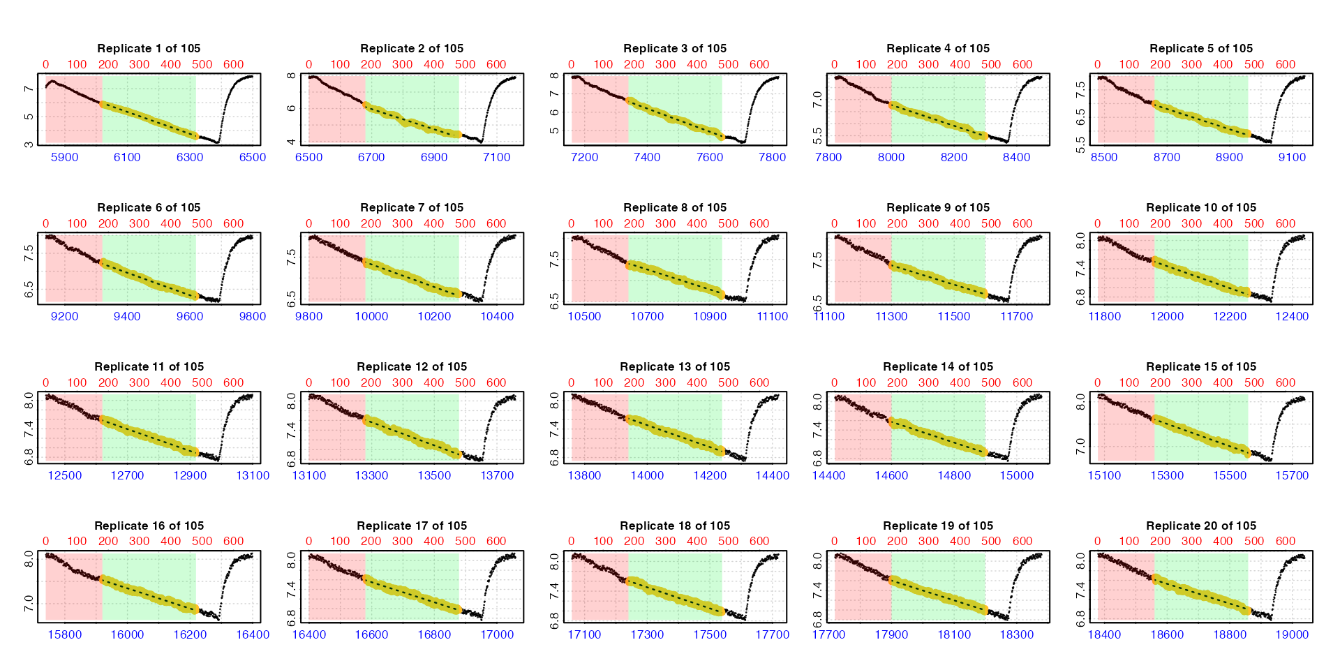 By default the function plots the first 20 replicates (
pos
can be used to choose others up to a maximum of 20). Note how the lower
time axis has the actual raw data time values, but the top row axis
refers to the rows of each replicate subset. In these plots the rate
data is the yellow points, the red shaded region is the
wait phase, and the green shaded region the
measure phase.
We can use summary() to view the results.
summary(zeb_cr.int)
#>
#> # summary.calc_rate.int # ---------------
#> Summary of all replicate results:
#>
#>      rep rank intercept_b0 slope_b1   rsq   row endrow  time endtime  oxy endoxy rate.2pt     rate
#>   1:   1    1         53.3 -0.00786 0.995   181    480  6020    6319 5.90   3.57 -0.00781 -0.00786
#>   2:   2    1         47.2 -0.00615 0.977   841   1140  6680    6979 6.24   4.41 -0.00614 -0.00615
#>   3:   3    1         52.7 -0.00628 0.990  1501   1800  7340    7639 6.64   4.64 -0.00668 -0.00628
#>   4:   4    1         41.3 -0.00432 0.984  2161   2460  8000    8299 6.74   5.45 -0.00434 -0.00432
#>   5:   5    1         38.8 -0.00368 0.986  2821   3120  8660    8959 6.99   5.88 -0.00369 -0.00368
#>  ---
#> 101: 101    1        162.7 -0.00215 0.974 66181  66480 72020   72319 7.58   6.94 -0.00215 -0.00215
#> 102: 102    1        174.1 -0.00229 0.977 66841  67140 72680   72979 7.56   6.88 -0.00228 -0.00229
#> 103: 103    1        168.4 -0.00219 0.977 67501  67800 73340   73639 7.59   6.94 -0.00217 -0.00219
#> 104: 104    1        181.5 -0.00235 0.977 68161  68460 74000   74299 7.62   6.93 -0.00231 -0.00235
#> 105: 105    1        170.0 -0.00218 0.972 68821  69120 74660   74959 7.61   6.96 -0.00218 -0.00218
#> -----------------------------------------
As we saw from our inspection of the data earlier, rates are higher at the start of the
dataset because the specimen was exercised before being placed in the
respirometer. We will filter these out shortly. For now we can see we
have a rate from every replicate. Our entered time range has been
applied within each replicate, and the replicate each rate
originates from can be seen in the $rep column.
Adjust
calc_rate.int objects also work with
adjust_rate, including with dynamic adjustment methods.
Here, we’ll adjust using the pre- and post-experiment background
recordings assuming the background rate increases linearly from the
initial to ending background rates.
zeb_cr.int_adj <- adjust_rate(zeb_cr.int,
                              by = bg_pre,
                              by2 = bg_post,
                              method = "linear")
#> adjust_rate: Rate adjustments applied using "linear" method.
If the adjustments were correctly applied we would expect the
adjustment value of the early replicates to be close to the value of the
initial background rate (-0.000074), and those of the later
ones close to that of the ending background rate
(-0.000120). Let’s look at the summary to check, and use
pos to pick out one from the start, middle and end.
summary(zeb_cr.int_adj, pos = c(1, 50, 105))
#>
#> # summary.adjust_rate # -----------------
#>
#> Adjustment was applied using 'linear' method.
#> Summary of rate results from entered 'pos' rank(s):
#>
#>    rep rank intercept_b0 slope_b1   rsq   row endrow  time endtime  oxy endoxy rate.2pt     rate adjustment rate.adjusted
#> 1:   1    1         53.3 -0.00786 0.995   181    480  6020    6319 5.90   3.57 -0.00781 -0.00786 -0.0000765      -0.00778
#> 2:  50    1         89.6 -0.00214 0.966 32521  32820 38360   38659 7.64   7.03 -0.00204 -0.00214 -0.0000971      -0.00204
#> 3: 105    1        170.0 -0.00218 0.972 68821  69120 74660   74959 7.61   6.96 -0.00218 -0.00218 -0.0001201      -0.00206
#> -----------------------------------------
As expected the $adjustment column values increase over
the experiment between these values, so we can proceed to
conversion.
Convert
Now we will convert the rates, then plot the values to decide how to select a final RMR rate.
zeb_cr.int_conv <- convert_rate(zeb_cr.int_adj,
                                oxy.unit = "mg/L",       # oxygen units of the original raw data
                                time.unit = "secs",      # time units of the original raw data
                                output.unit = "mg/h/g",  # desired output unit
                                volume = 0.12,           # effective volume of the respirometer in L
                                mass = 0.0009)           # mass of the specimen in kg
The converted rates can be seen in the summary table.
summary(zeb_cr.int_conv)
#>
#> # summary.convert_rate # ----------------
#> Summary of all converted rates:
#>
#>      rep rank intercept_b0 slope_b1   rsq density   row endrow  time endtime  oxy endoxy     rate adjustment rate.adjusted rate.input oxy.unit time.unit volume   mass area  S  t  P rate.abs rate.m.spec rate.a.spec output.unit rate.output
#>   1:   1    1         53.3 -0.00786 0.995      NA   181    480  6020    6319 5.90   3.57 -0.00786 -0.0000765      -0.00778   -0.00778     mg/L       sec   0.12 0.0009   NA NA NA NA   -3.363      -3.736          NA   mgO2/hr/g      -3.736
#>   2:   2    1         47.2 -0.00615 0.977      NA   841   1140  6680    6979 6.24   4.41 -0.00615 -0.0000769      -0.00608   -0.00608     mg/L       sec   0.12 0.0009   NA NA NA NA   -2.625      -2.917          NA   mgO2/hr/g      -2.917
#>   3:   3    1         52.7 -0.00628 0.990      NA  1501   1800  7340    7639 6.64   4.64 -0.00628 -0.0000773      -0.00621   -0.00621     mg/L       sec   0.12 0.0009   NA NA NA NA   -2.681      -2.978          NA   mgO2/hr/g      -2.978
#>   4:   4    1         41.3 -0.00432 0.984      NA  2161   2460  8000    8299 6.74   5.45 -0.00432 -0.0000778      -0.00424   -0.00424     mg/L       sec   0.12 0.0009   NA NA NA NA   -1.831      -2.035          NA   mgO2/hr/g      -2.035
#>   5:   5    1         38.8 -0.00368 0.986      NA  2821   3120  8660    8959 6.99   5.88 -0.00368 -0.0000782      -0.00360   -0.00360     mg/L       sec   0.12 0.0009   NA NA NA NA   -1.556      -1.729          NA   mgO2/hr/g      -1.729
#>  ---
#> 101: 101    1        162.7 -0.00215 0.974      NA 66181  66480 72020   72319 7.58   6.94 -0.00215 -0.0001185      -0.00203   -0.00203     mg/L       sec   0.12 0.0009   NA NA NA NA   -0.879      -0.977          NA   mgO2/hr/g      -0.977
#> 102: 102    1        174.1 -0.00229 0.977      NA 66841  67140 72680   72979 7.56   6.88 -0.00229 -0.0001189      -0.00217   -0.00217     mg/L       sec   0.12 0.0009   NA NA NA NA   -0.939      -1.043          NA   mgO2/hr/g      -1.043
#> 103: 103    1        168.4 -0.00219 0.977      NA 67501  67800 73340   73639 7.59   6.94 -0.00219 -0.0001193      -0.00207   -0.00207     mg/L       sec   0.12 0.0009   NA NA NA NA   -0.895      -0.995          NA   mgO2/hr/g      -0.995
#> 104: 104    1        181.5 -0.00235 0.977      NA 68161  68460 74000   74299 7.62   6.93 -0.00235 -0.0001197      -0.00223   -0.00223     mg/L       sec   0.12 0.0009   NA NA NA NA   -0.963      -1.070          NA   mgO2/hr/g      -1.070
#> 105: 105    1        170.0 -0.00218 0.972      NA 68821  69120 74660   74959 7.61   6.96 -0.00218 -0.0001201      -0.00206   -0.00206     mg/L       sec   0.12 0.0009   NA NA NA NA   -0.888      -0.987          NA   mgO2/hr/g      -0.987
#> -----------------------------------------
We can see the converted rates as the last column. The
$summary table contains the all rate regression parameters
and data locations, adjustments (if applied), units, and more. It can be
exported as a separate data frame by using export = TRUE in
summary(). This is a great way of exporting all the
relevant data for your final results.
Select
It will depend on the aims and circumstances of an experiment what rate results to extract, summarise, and report. For instance we might report RMR as a mean of a representative selection of rates after the specimens uptake rate has stabilised, or a mean of a number or percentile of lowest rates found. The important thing is to apply these selection criteria consistently and report them alongside results.
As of respR v2.1
convert_rate has new plotting functionality to help
visualise and explore rate results. For intermittent-flow results the
most useful of these is type = "rate".
plot(zeb_cr.int_conv, type = "rate")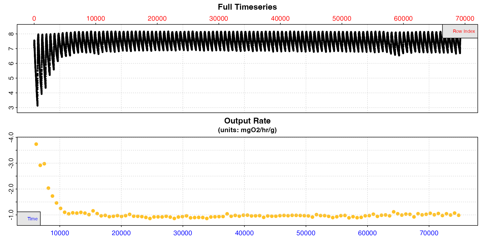
This shows how the calculated rate values vary across the dataset. We can see from this plot they are high at the start, stabilise after around timepoint 20000, then are a little unstable again if not slightly elevated after timepoint 60000. Between these however they appear to be very stable.
The select_rate() function allows
convert_rate results to be filtered or reordered in various
ways. See help("select_rate") and
vignette("select_rate") for more details. For this
analysis, lets only use rates from replicates between timepoints 20000
and 60000. Then, simply to show an example of how rates can be further
selected, let’s only select those with r-squared of 0.97 and above,
select the lowest 20, and finally take the mean of them.
RMR <- zeb_cr.int_conv |>
  select_rate(method = "time", n = c(20000, 60000)) |>
  select_rate(method = "rsq", n = c(0.97, 1)) |>
  select_rate(method = "lowest", n = 20) |>
  summary() |>
  mean()
#> select_rate: Selecting rates which occur only between times 20000 and 60000...
#> ----- Selection complete. 45 rate(s) removed, 60 rate(s) remaining -----
#> select_rate: Selecting rates with rsq values between 0.97 and 1...
#> ----- Selection complete. 24 rate(s) removed, 36 rate(s) remaining -----
#> select_rate: Selecting lowest 20 *absolute* rate values...
#> ----- Selection complete. 16 rate(s) removed, 20 rate(s) remaining -----
#>
#> # summary.convert_rate # ----------------
#> Summary of all converted rates:
#>
#>     rep rank intercept_b0 slope_b1   rsq density   row endrow  time endtime  oxy endoxy     rate adjustment rate.adjusted rate.input oxy.unit time.unit volume   mass area  S  t  P rate.abs rate.m.spec rate.a.spec output.unit rate.output
#>  1:  25    1         52.8 -0.00207 0.971      NA 16021  16320 21860   22159 7.70   7.06 -0.00207 -0.0000866      -0.00198   -0.00198     mg/L       sec   0.12 0.0009   NA NA NA NA   -0.855      -0.950          NA   mgO2/hr/g      -0.950
#>  2:  26    1         54.0 -0.00206 0.972      NA 16681  16980 22520   22819 7.68   7.06 -0.00206 -0.0000870      -0.00197   -0.00197     mg/L       sec   0.12 0.0009   NA NA NA NA   -0.851      -0.946          NA   mgO2/hr/g      -0.946
#>  3:  33    1         63.6 -0.00206 0.972      NA 21301  21600 27140   27439 7.71   7.08 -0.00206 -0.0000899      -0.00197   -0.00197     mg/L       sec   0.12 0.0009   NA NA NA NA   -0.852      -0.947          NA   mgO2/hr/g      -0.947
#>  4:  36    1         66.0 -0.00200 0.971      NA 23281  23580 29120   29419 7.66   7.08 -0.00200 -0.0000912      -0.00191   -0.00191     mg/L       sec   0.12 0.0009   NA NA NA NA   -0.826      -0.917          NA   mgO2/hr/g      -0.917
#>  5:  38    1         71.5 -0.00210 0.972      NA 24601  24900 30440   30739 7.63   7.06 -0.00210 -0.0000920      -0.00201   -0.00201     mg/L       sec   0.12 0.0009   NA NA NA NA   -0.867      -0.963          NA   mgO2/hr/g      -0.963
#>  6:  39    1         68.0 -0.00194 0.971      NA 25261  25560 31100   31399 7.71   7.05 -0.00194 -0.0000924      -0.00185   -0.00185     mg/L       sec   0.12 0.0009   NA NA NA NA   -0.799      -0.887          NA   mgO2/hr/g      -0.887
#>  7:  49    1         85.7 -0.00207 0.972      NA 31861  32160 37700   37999 7.69   7.03 -0.00207 -0.0000966      -0.00197   -0.00197     mg/L       sec   0.12 0.0009   NA NA NA NA   -0.853      -0.947          NA   mgO2/hr/g      -0.947
#>  8:  51    1         88.7 -0.00208 0.970      NA 33181  33480 39020   39319 7.66   6.98 -0.00208 -0.0000975      -0.00198   -0.00198     mg/L       sec   0.12 0.0009   NA NA NA NA   -0.856      -0.951          NA   mgO2/hr/g      -0.951
#>  9:  55    1         95.4 -0.00211 0.973      NA 35821  36120 41660   41959 7.63   7.03 -0.00211 -0.0000992      -0.00201   -0.00201     mg/L       sec   0.12 0.0009   NA NA NA NA   -0.868      -0.964          NA   mgO2/hr/g      -0.964
#> 10:  58    1         99.3 -0.00210 0.973      NA 37801  38100 43640   43939 7.70   7.04 -0.00210 -0.0001004      -0.00200   -0.00200     mg/L       sec   0.12 0.0009   NA NA NA NA   -0.864      -0.960          NA   mgO2/hr/g      -0.960
#> 11:  59    1         99.7 -0.00208 0.971      NA 38461  38760 44300   44599 7.66   6.95 -0.00208 -0.0001008      -0.00198   -0.00198     mg/L       sec   0.12 0.0009   NA NA NA NA   -0.855      -0.950          NA   mgO2/hr/g      -0.950
#> 12:  63    1        107.2 -0.00212 0.977      NA 41101  41400 46940   47239 7.63   7.00 -0.00212 -0.0001025      -0.00202   -0.00202     mg/L       sec   0.12 0.0009   NA NA NA NA   -0.872      -0.969          NA   mgO2/hr/g      -0.969
#> 13:  68    1        113.5 -0.00211 0.971      NA 44401  44700 50240   50539 7.67   7.02 -0.00211 -0.0001046      -0.00200   -0.00200     mg/L       sec   0.12 0.0009   NA NA NA NA   -0.865      -0.962          NA   mgO2/hr/g      -0.962
#> 14:  73    1        118.7 -0.00207 0.972      NA 47701  48000 53540   53839 7.67   7.01 -0.00207 -0.0001067      -0.00197   -0.00197     mg/L       sec   0.12 0.0009   NA NA NA NA   -0.850      -0.944          NA   mgO2/hr/g      -0.944
#> 15:  74    1        114.6 -0.00197 0.970      NA 48361  48660 54200   54499 7.66   7.02 -0.00197 -0.0001071      -0.00187   -0.00187     mg/L       sec   0.12 0.0009   NA NA NA NA   -0.807      -0.896          NA   mgO2/hr/g      -0.896
#> 16:  75    1        119.6 -0.00204 0.973      NA 49021  49320 54860   55159 7.67   7.04 -0.00204 -0.0001076      -0.00193   -0.00193     mg/L       sec   0.12 0.0009   NA NA NA NA   -0.835      -0.928          NA   mgO2/hr/g      -0.928
#> 17:  79    1        125.3 -0.00205 0.973      NA 51661  51960 57500   57799 7.67   7.04 -0.00205 -0.0001092      -0.00194   -0.00194     mg/L       sec   0.12 0.0009   NA NA NA NA   -0.837      -0.930          NA   mgO2/hr/g      -0.930
#> 18:  80    1        122.0 -0.00197 0.971      NA 52321  52620 58160   58459 7.60   7.01 -0.00197 -0.0001097      -0.00186   -0.00186     mg/L       sec   0.12 0.0009   NA NA NA NA   -0.803      -0.892          NA   mgO2/hr/g      -0.892
#> 19:  81    1        125.0 -0.00200 0.974      NA 52981  53280 58820   59119 7.67   7.01 -0.00200 -0.0001101      -0.00189   -0.00189     mg/L       sec   0.12 0.0009   NA NA NA NA   -0.815      -0.905          NA   mgO2/hr/g      -0.905
#> 20:  82    1        133.8 -0.00212 0.973      NA 53641  53940 59480   59779 7.68   7.03 -0.00212 -0.0001105      -0.00201   -0.00201     mg/L       sec   0.12 0.0009   NA NA NA NA   -0.869      -0.965          NA   mgO2/hr/g      -0.965
#> -----------------------------------------
#>
#> # mean.convert_rate # -------------------
#> Mean of all rate results:
#>
#> Mean of 20 output rates:
#> [1] -0.939
#> [1] "mgO2/hr/g"
#> -----------------------------------------
That’s it; this is our final routine metabolic rate (at least, as we have chosen to define it).
SMR
auto_rate.int
To extract a rate from every replicate and determine a standard
metabolic rate (SMR) from amongst the results we will use
auto_rate.int(). To repeat the note from above, this is not a recommendation that this is
how you should extract an SMR from your own data; it is simply an
example of one approach and how the respR functions are
flexible and adaptable.
Introduced in respR v2.1,
auto_rate.int() is a dedicated function for
intermittent-flow respirometry data, in which you specify a replicate
structure and run auto_rate() on each replicate. This
function extracts rates in a number of ways including the most linear or
most consistently maintained rates, plus highest and lowest rates of a
specified width. See vignette("auto_rate") for more
details, and vignette("auto_rate.int") for an overview of
this function.
The difference between this and the approach above using calc_rate.int() is that the
specified measure phase is not the same as the region over
which a rate is calculated. Instead a measure phase is
specified and the auto_rate analysis is done
within this region using the method and
width inputs. This can result in rates of different widths
coming from within this region depending on the inputs.
Subset data
We again subset the data so that the 105 regularly-spaced replicates start at row 1.
zeb_insp <- zeb_intermittent.rd |>
  subset_data(from = 5840,
              to = 75139,
              by = "row") |>
  inspect()
#> inspect: Applying column default of 'time = 1'
#> inspect: Applying column default of 'oxygen = 2'
#> inspect: No issues detected while inspecting data frame.
Extract rates
To get SMR we necessarily need to define it, in particular the duration over which rates are calculated within each replicate. These should be chosen appropriately and with reference to best practices and previous studies. Here, let’s say we want to extract the lowest rate across 2 minutes within each replicate, and we will define our SMR for this specimen as the mean of the lowest 10th percentile of all 105 extracted rates.
We run auto_rate.int on the inspected data and use
method = "lowest" and width = 120. This means
the function calculates every rate of this width within each
replicate, orders them according to the input method, and
by default (n = 1) returns the top ranked result, in this
case the lowest, for each replicate.
We again specify a 660 row interval between replicates using
starts. Just to be different from the above example, this time we will specify a 2 minute
(120 row) wait phase, and six minute (360 row)
measure phase.
zeb_ar.int <- auto_rate.int(zeb_insp,
                            starts = 660,
                            wait = 120,
                            measure = 360,
                            method = "lowest",
                            width = 120,
                            by = "row") |>
  summary()
#> plot.auto_rate.int: Plotting first 20 selected rates only. To plot others modify 'pos' input.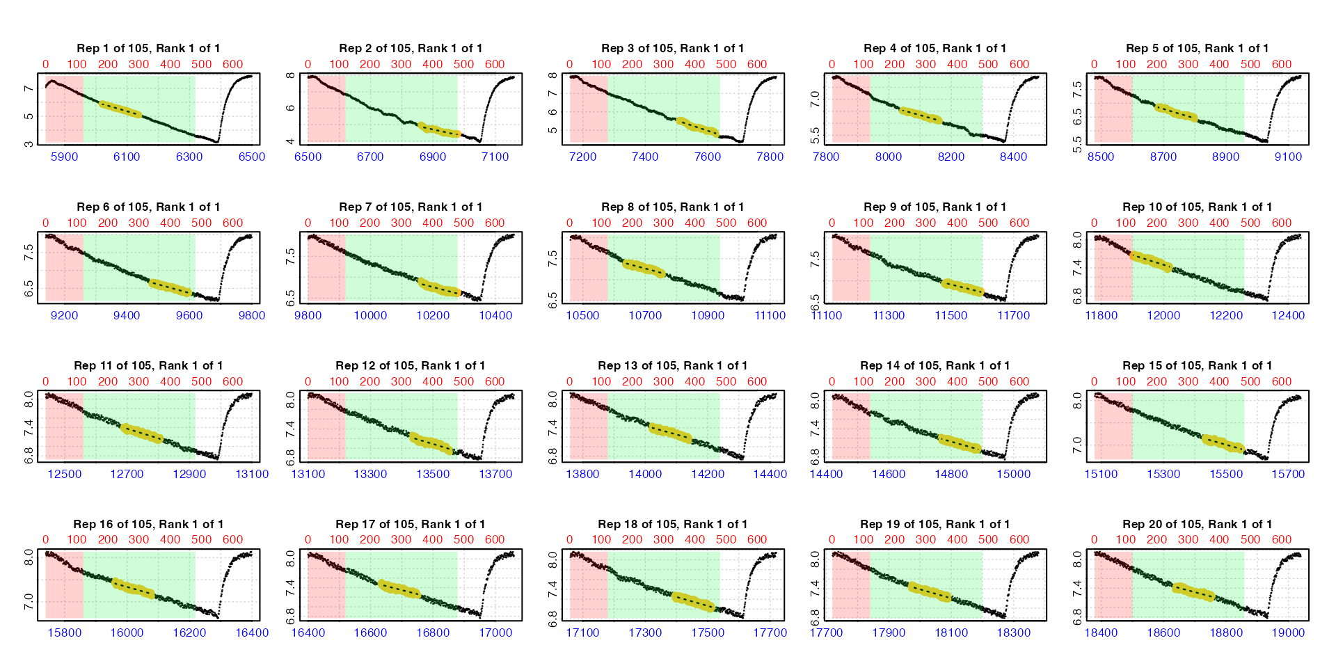
Note how the plots show the rates coming from different regions within each replicate measure phase. The summary contains all the results, that is the lowest 2-minute rate from each replicate. Before selecting from amongst these to get our final SMR we first need to adjust and convert them. This is exactly the same process we followed in the example above.
Adjust
zeb_ar.int_adj <- adjust_rate(zeb_ar.int,
                              by = bg_pre,
                              by2 = bg_post,
                              method = "linear")
#> adjust_rate: Rate adjustments applied using "linear" method.
Convert
zeb_ar.int_conv <- convert_rate(zeb_ar.int_adj,
                                oxy.unit = "mg/L",       # oxygen units of the original raw data
                                time.unit = "secs",      # time units of the original raw data
                                output.unit = "mg/h/g",  # desired output unit
                                volume = 0.12,           # effective volume of the respirometer in L
                                mass = 0.0009)           # mass of the specimen in kg
summary(zeb_ar.int_conv)
#>
#> # summary.convert_rate # ----------------
#> Summary of all converted rates:
#>
#>      rep rank intercept_b0 slope_b1   rsq density   row endrow  time endtime  oxy endoxy     rate adjustment rate.adjusted rate.input oxy.unit time.unit volume   mass area  S  t  P rate.abs rate.m.spec rate.a.spec output.unit rate.output
#>   1:   1    1         45.5 -0.00658 0.984      NA   179    298  6018    6137 5.88   5.12 -0.00658 -0.0000764      -0.00650   -0.00650     mg/L       sec   0.12 0.0009   NA NA NA NA   -2.810      -3.122          NA   mgO2/hr/g      -3.122
#>   2:   2    1         34.0 -0.00424 0.906      NA  1021   1140  6860    6979 5.00   4.41 -0.00424 -0.0000770      -0.00416   -0.00416     mg/L       sec   0.12 0.0009   NA NA NA NA   -1.798      -1.998          NA   mgO2/hr/g      -1.998
#>   3:   3    1         47.3 -0.00557 0.932      NA  1668   1787  7507    7626 5.51   4.81 -0.00557 -0.0000774      -0.00549   -0.00549     mg/L       sec   0.12 0.0009   NA NA NA NA   -2.374      -2.638          NA   mgO2/hr/g      -2.638
#>   4:   4    1         35.5 -0.00360 0.952      NA  2203   2322  8042    8161 6.55   6.13 -0.00360 -0.0000777      -0.00352   -0.00352     mg/L       sec   0.12 0.0009   NA NA NA NA   -1.522      -1.691          NA   mgO2/hr/g      -1.691
#>   5:   5    1         36.2 -0.00338 0.928      NA  2841   2960  8680    8799 6.87   6.50 -0.00338 -0.0000781      -0.00330   -0.00330     mg/L       sec   0.12 0.0009   NA NA NA NA   -1.426      -1.584          NA   mgO2/hr/g      -1.584
#>  ---
#> 101: 101    1        154.6 -0.00204 0.850      NA 66251  66370 72090   72209 7.43   7.20 -0.00204 -0.0001185      -0.00192   -0.00192     mg/L       sec   0.12 0.0009   NA NA NA NA   -0.831      -0.923          NA   mgO2/hr/g      -0.923
#> 102: 102    1        146.2 -0.00191 0.836      NA 66862  66981 72701   72820 7.54   7.32 -0.00191 -0.0001188      -0.00179   -0.00179     mg/L       sec   0.12 0.0009   NA NA NA NA   -0.773      -0.859          NA   mgO2/hr/g      -0.859
#> 103: 103    1        151.7 -0.00197 0.852      NA 67680  67799 73519   73638 7.18   6.97 -0.00197 -0.0001194      -0.00185   -0.00185     mg/L       sec   0.12 0.0009   NA NA NA NA   -0.797      -0.886          NA   mgO2/hr/g      -0.886
#> 104: 104    1        162.6 -0.00209 0.864      NA 68269  68388 74108   74227 7.35   7.10 -0.00209 -0.0001197      -0.00197   -0.00197     mg/L       sec   0.12 0.0009   NA NA NA NA   -0.853      -0.948          NA   mgO2/hr/g      -0.948
#> 105: 105    1        147.5 -0.00187 0.817      NA 68986  69105 74825   74944 7.17   6.97 -0.00187 -0.0001202      -0.00175   -0.00175     mg/L       sec   0.12 0.0009   NA NA NA NA   -0.758      -0.842          NA   mgO2/hr/g      -0.842
#> -----------------------------------------
Quality control
We can plot the convert_rate object for a quick look at
how rates vary across the data.
plot(zeb_ar.int_conv, type = "rate")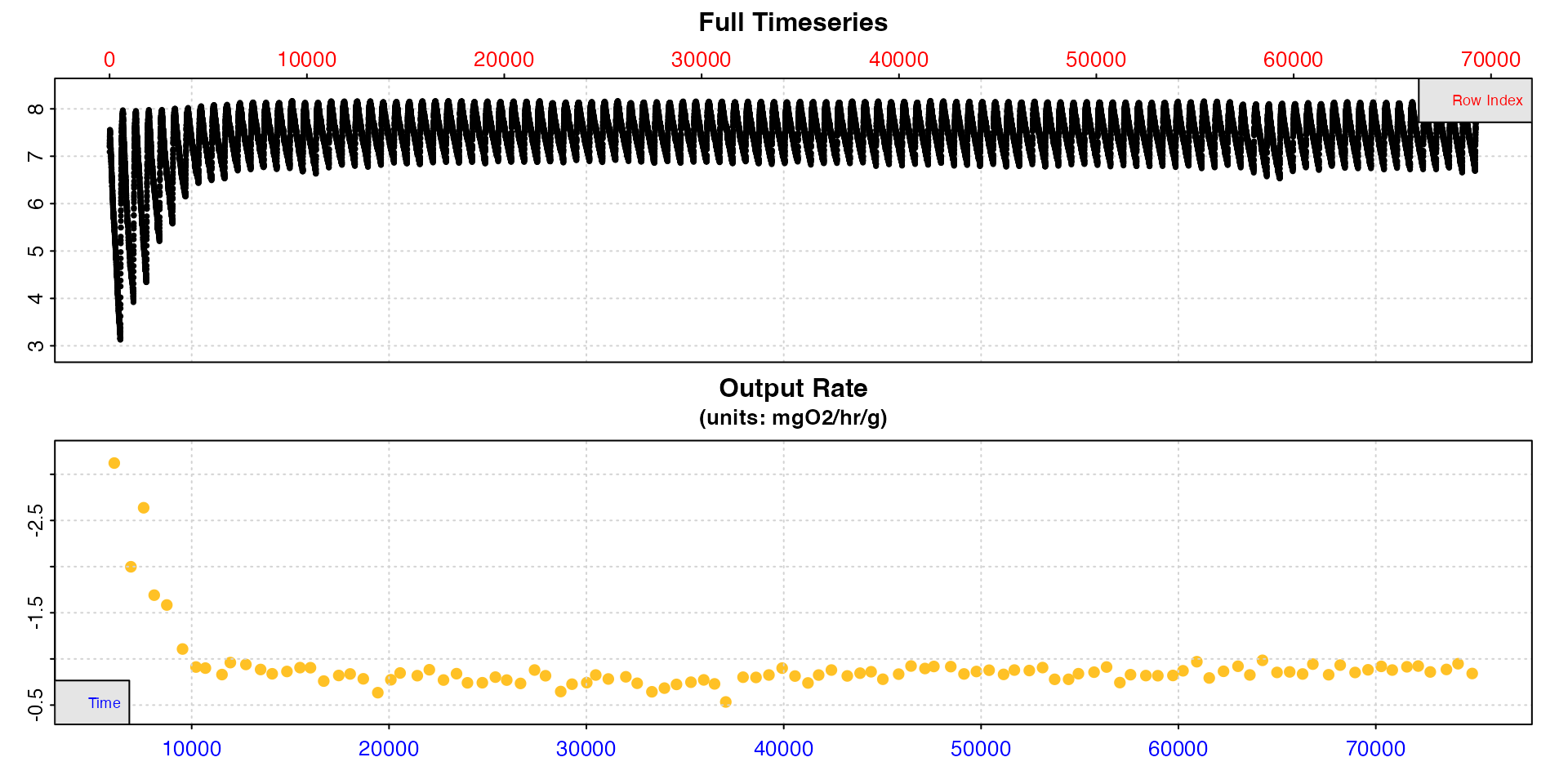
These rates seem to be a bit lower than those we extracted for RMR above, as we would expect for an SMR.
This is an opportunity to do some quality control before we select
our final rates to determine SMR. Looking at the plot above there is one
result that seems to be uncharacteristically low compared to the others
with a value just over 0.5. Looking at the summary table we can see this
is from replicate 48. We can plot a selection of rates from this region
using pos and the y-axis range will adapt to provide a more
detailed view of the range of rates.
plot(zeb_ar.int_conv, type = "rate", pos = 30:80)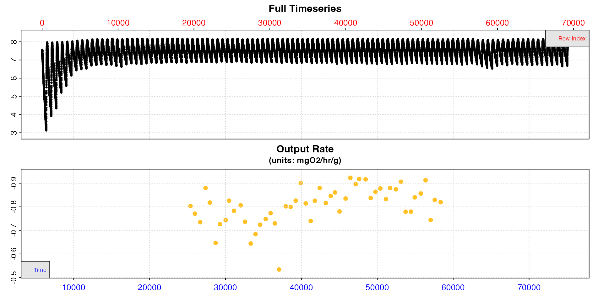
Replicate 48 does seem to be anomalously low. If we go back to the
auto_rate.int results object we can use pos to
plot this replicate for a closer look. We’ll do this in two different
ways using type. Firstly the rate in the context of the
whole replicate, secondly the auto_rate output plot for
this replicate which has more diagnostic plots, but only shows the
measure phase.
plot(zeb_ar.int, type = "rep", pos = 48)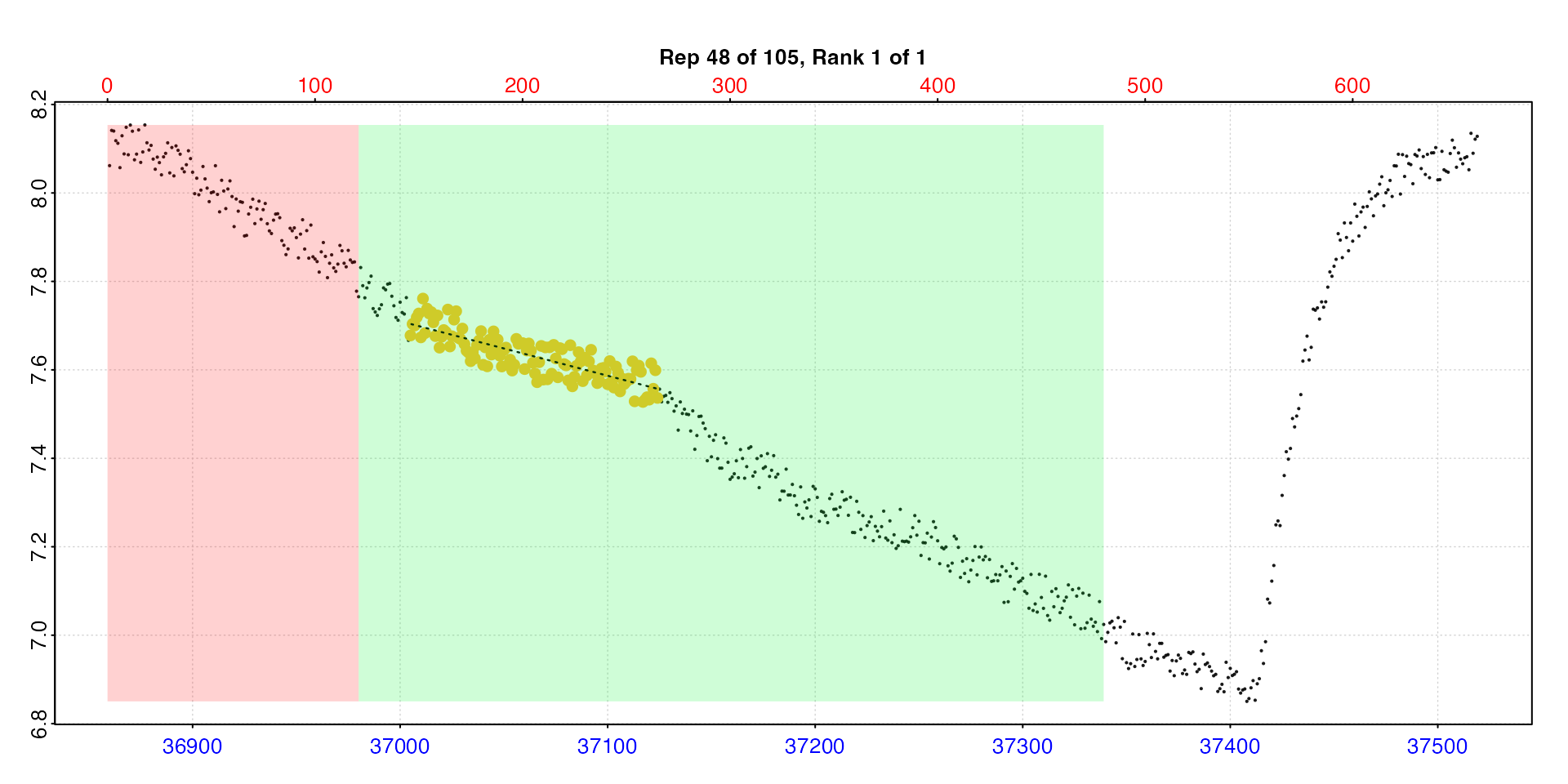
plot(zeb_ar.int, type = "ar", pos = 48)
Looking at these plots this result does seem to be anomalous, and in this replicate the rate extracted is not really representative. It also has a lower r-squared which otherwise varies from 0.72 to 0.98. There seems to be an anomaly in the oxygen trace, maybe a sensor glitch or slight temperature change. Issues like this causing glitches in the trace are very common.
Therefore, it would be perfectly acceptable and justifiable to manually exclude this result (there are also 1 or 2 others we might want to investigate). To apply such selection criteria objectively and systematically would require examining multiple experiments. This is why definitions of metrics like SMR and analysis parameters should usually be decided upon after thoroughly exploring all your results. After this you should be able to arrive at a set of objective and reasonable selection criteria.
Select
To get our final SMR we just need to use select_rate
again with our chosen criteria, and pipe the result to
mean. We decided above our
definition of SMR would be the mean of the lowest 10th percentile of the
rates extracted from each replicate. We also want to exclude the result
from replicate 48.
Excluding this replicate could be achieved in a number of ways in
select_rate. We could use method = "rsq" to
select only results with r-squared above a certain value which excludes
this one. We could use the time_omit method to exclude this
rate based on its timepoint (found in the summary table), or use the
rep method simply to select all replicates except
this one. There is a specific rep_omit method however to
remove particular replicates.
SMR <- zeb_ar.int_conv |>
  select_rate(method = "rep_omit", n = 48) |>
  select_rate(method = "lowest_percentile", n = 0.1) |>
  summary() |>
  mean()
#> select_rate: Selecting rates which *ARE NOT* from 'rep_omit' replicates...
#> ----- Selection complete. 1 rate(s) removed, 104 rate(s) remaining -----
#> select_rate: Selecting lowest 10th percentile of *absolute* rate values...
#> ----- Selection complete. 93 rate(s) removed, 11 rate(s) remaining -----
#>
#> # summary.convert_rate # ----------------
#> Summary of all converted rates:
#>
#>     rep rank intercept_b0 slope_b1   rsq density   row endrow  time endtime  oxy endoxy     rate adjustment rate.adjusted rate.input oxy.unit time.unit volume   mass area  S  t  P rate.abs rate.m.spec rate.a.spec output.unit rate.output
#>  1:  21    1         34.5 -0.00141 0.725      NA 13533  13652 19372   19491 7.24   7.12 -0.00141 -0.0000849      -0.00132   -0.00132     mg/L       sec   0.12 0.0009   NA NA NA NA   -0.571      -0.634          NA   mgO2/hr/g      -0.634
#>  2:  28    1         46.5 -0.00163 0.789      NA 18076  18195 23915   24034 7.45   7.29 -0.00163 -0.0000878      -0.00154   -0.00154     mg/L       sec   0.12 0.0009   NA NA NA NA   -0.667      -0.741          NA   mgO2/hr/g      -0.741
#>  3:  32    1         50.5 -0.00162 0.802      NA 20764  20883 26603   26722 7.38   7.16 -0.00162 -0.0000895      -0.00153   -0.00153     mg/L       sec   0.12 0.0009   NA NA NA NA   -0.661      -0.735          NA   mgO2/hr/g      -0.735
#>  4:  35    1         48.4 -0.00144 0.722      NA 22801  22920 28640   28759 7.27   7.11 -0.00144 -0.0000908      -0.00135   -0.00135     mg/L       sec   0.12 0.0009   NA NA NA NA   -0.582      -0.647          NA   mgO2/hr/g      -0.647
#>  5:  36    1         54.4 -0.00160 0.783      NA 23373  23492 29212   29331 7.50   7.31 -0.00160 -0.0000912      -0.00151   -0.00151     mg/L       sec   0.12 0.0009   NA NA NA NA   -0.654      -0.726          NA   mgO2/hr/g      -0.726
#>  6:  41    1         60.3 -0.00163 0.780      NA 26675  26794 32514   32633 7.36   7.25 -0.00163 -0.0000933      -0.00153   -0.00153     mg/L       sec   0.12 0.0009   NA NA NA NA   -0.663      -0.736          NA   mgO2/hr/g      -0.736
#>  7:  42    1         55.0 -0.00144 0.727      NA 27421  27540 33260   33379 7.26   7.11 -0.00144 -0.0000938      -0.00134   -0.00134     mg/L       sec   0.12 0.0009   NA NA NA NA   -0.580      -0.644          NA   mgO2/hr/g      -0.644
#>  8:  43    1         58.8 -0.00152 0.776      NA 28056  28175 33895   34014 7.28   7.14 -0.00152 -0.0000942      -0.00142   -0.00142     mg/L       sec   0.12 0.0009   NA NA NA NA   -0.615      -0.684          NA   mgO2/hr/g      -0.684
#>  9:  44    1         62.7 -0.00160 0.775      NA 28667  28786 34506   34625 7.37   7.20 -0.00160 -0.0000946      -0.00151   -0.00151     mg/L       sec   0.12 0.0009   NA NA NA NA   -0.652      -0.724          NA   mgO2/hr/g      -0.724
#> 10:  47    1         66.4 -0.00162 0.792      NA 30595  30714 36434   36553 7.54   7.32 -0.00162 -0.0000958      -0.00152   -0.00152     mg/L       sec   0.12 0.0009   NA NA NA NA   -0.657      -0.730          NA   mgO2/hr/g      -0.730
#> 11:  54    1         74.8 -0.00164 0.766      NA 35329  35448 41168   41287 7.21   7.02 -0.00164 -0.0000988      -0.00154   -0.00154     mg/L       sec   0.12 0.0009   NA NA NA NA   -0.666      -0.740          NA   mgO2/hr/g      -0.740
#> -----------------------------------------
#>
#> # mean.convert_rate # -------------------
#> Mean of all rate results:
#>
#> Mean of 11 output rates:
#> [1] -0.704
#> [1] "mgO2/hr/g"
#> -----------------------------------------
We can see the summary of the final 11 selected rates, and then the mean of these. This is our final SMR.
Summary
Now we have our final results for each metric.
Typically these rates would now be reported as positive values.
Reporting
The above is a lengthy description of an analysis, so this vignette
may not give a good impression of just how succinct a respR
analysis may be. This code block shows the entire analysis for SMR.
Complete analysis
# Inspect data ------------------------------------------------------------
zeb <- inspect(zeb_intermittent.rd)

# Background --------------------------------------------------------------
bg_pre <- subset_data(zeb, from = 0, to = 4999, by = "time") |>
  calc_rate.bg()
bg_post <- subset_data(zeb, from = 75140, to = 79251, by = "time") |>
  calc_rate.bg()

# SMR Analysis ------------------------------------------------------------
  # Subset ------------------------------------------------------------------
  zeb |>
  subset_data(from = 5840,
              to = 75139,
              by = "row") |>
  # Extract rates -----------------------------------------------------------
  auto_rate.int(starts = 660,
                wait = 120,
                measure = 360,
                method = "lowest",
                width = 120,
                by = "row")  |>
  # Adjust ------------------------------------------------------------------
  adjust_rate(by = bg_pre,
              by2 = bg_post,
              method = "linear") |>
  # Convert -----------------------------------------------------------------
  convert_rate(oxy.unit = "mg/L",
               time.unit = "secs",
               output.unit = "mg/h/g",
               volume = 0.12,
               mass = 0.0009) |>
  # Select -----------------------------------------------------------------
  select_rate(method = "rep_omit", n = 48) |>
  select_rate(method = "lowest_percentile", n = 0.1) |>
  summary() |>
  mean()
How to report analysis methods
The ultimate aim of respR was to enable clear reporting
and reproducible analyses. This is an example of how we might report the
above analysis in a manuscript.
“Data was analysed using the R package respR
(Harianto et al. 2019). The auto_rate.int function was used
to extract the lowest rate across a two minute window from each
replicate. Rates were adjusted for background using pre- and
post-experiment blank recordings with no specimen, assuming a linear
increase in background rate over time. Obviously anomalous rates were
excluded, and SMR was defined as the mean of the lowest 10th percentile
of remaining adjusted rates.”
Alternative approaches
Previous versions of this vignette demonstrated use of different
methods, such as looping and subsetting of data, to extract individual
replicates for processing through calc_rate or
auto_rate. These approaches still work and are archived here
in case they are of use in some cases, for example if you want to
extract rates from the same oxygen range in each replicate. However for
most analyses use of calc_rate.int or
auto_rate.int is the recommended approach.