Automatically determine most linear, highest, lowest and rolling oxygen uptake or production rates
Source:R/auto_rate.R
auto_rate.Rdauto_rate performs rolling regressions on a dataset to determine the most
linear, highest, lowest, maximum, minimum, rolling, and interval rates of
change in oxygen against time. A rolling regression of the specified width
is performed on the entire dataset, then based on the "method" input, the
resulting regressions are ranked or ordered, and the output summarised.
Arguments
- x
data frame, or object of class
inspectcontaining oxygen~time data.- method
string.
"linear","highest","lowest","maximum","minimum","rolling"or"interval". Defaults to"linear". See Details.- width
numeric. Width of the rolling regression. For
by = "row", either a value between 0 and 1 representing a proportion of the data length, or an integer of 2 or greater representing an exact number of rows. Ifby = "time"it represents a time window in the units of the time data. IfNULL, it defaults to 0.2 or a window of 20% of the data length. See Details.- by
string.
"row"or"time". Defaults to"row". Metric by which to apply thewidthinput if it is above 1.- plot
logical. Defaults to TRUE. Plot the results.
- ...
Allows additional plotting controls to be passed, such as
pos,panel, andquiet = TRUE.
Value
Output is a list object of class auto_rate containing input
parameters and data, various summary data, metadata, linear models, and the
primary output of interest $rate, which can be background adjusted in
adjust_rate or converted to units in convert_rate.
Details
Ranking and ordering algorithms
Currently, auto_rate contains seven ranking and ordering algorithms that
can be applied using the method input:
linear: Uses kernel density estimation (KDE) to learn the shape of the entire dataset and automatically identify the most linear regions of the timeseries. This is achieved by using the smoothing bandwidth of the KDE to re-sample the "peaks" in the KDE to determine linear regions of the data. The summary output will contain only the regressions identified as coming from linear regions of the data, ranked by order of the KDE density analysis. This is present in the$summarycomponent of the output as$density. Under this method, thewidthinput is used as a starting seed value, but the resulting regressions may be of any width. See here for full details.highest: Every regression of the specifiedwidthacross the entire timeseries is calculated, then ordered using absolute rate values from highest to lowest. Essentially, this option ignores the sign of the rate, and can only be used when rates all have the same sign. Rates will be ordered from highest to lowest in the$summarytable regardless of if they are oxygen uptake or oxygen production rates.lowest: Every regression of the specifiedwidthacross the entire timeseries is calculated, then ordered using absolute rate values from lowest to highest. Essentially, this option ignores the sign of the rate, and can only be used when rates all have the same sign. Rates will be ordered from lowest to highest in the$summarytable regardless of if they are oxygen uptake or oxygen production rates.maximum: Every regression of the specifiedwidthacross the entire timeseries is calculated, then ordered using numerical rate values from maximum to minimum. Takes full account of the sign of the rate. Therefore, oxygen uptake rates, which inrespRare negative, would be ordered from lowest (least negative), to highest (most negative) in the summary table in numerical order. Therefore, generally this method should only be used when rates are a mix of oxygen consumption and production rates, such as when positive rates may result from regressions fit over flush periods in intermittent-flow respirometry. Generally, for most analyses where maximum or minimum rates are of interest the"highest"or"lowest"methods should be used.minimum: Every regression of the specifiedwidthacross the entire timeseries is calculated, then ordered using numerical rate values from minimum to maximum. Takes full account of the sign of the rate. Therefore, oxygen uptake rates, which inrespRare negative, would be ordered from highest (most negative) to lowest (least negative) in the summary table in numerical order. Therefore, generally this method should only be used when rates are a mix of oxygen consumption and production rates, such as when positive rates may result from regressions fit over flush periods in intermittent-flow respirometry. Generally, for most analyses where maximum or minimum rates are of interest the"highest"or"lowest"methods should be used.rolling: A rolling regression of the specifiedwidthis performed across the entire timeseries. No reordering of results is performed.interval: multiple, successive, non-overlapping regressions of the specifiedwidthare extracted from the rolling regressions, ordered by time.
Further selection and filtering of results
For further selection or subsetting of auto_rate results, see the dedicated
select_rate() function, which allows subsetting of rates by various
criteria, including r-squared, data region, percentiles, and more.
Units
There are no units involved in auto_rate. This is a deliberate decision.
The units of oxygen concentration and time will be specified later in
convert_rate() when rates are converted to specific output units.
The width and by inputs
If by = "time", the width input represents a time window in the units of
the time data in x.
If by = "row" and width is between 0 and 1 it represents a proportion of
the total data length, as in the equation floor(width * number of data rows). For example, 0.2 represents a rolling window of 20% of the data
width. Otherwise, if entered as an integer of 2 or greater, the width
represents the number of rows.
For both by inputs, if left as width = NULL it defaults to 0.2 or a
window of 20% of the data length.
In most cases, by should be left as the default "row", and the width
chosen with this in mind, as it is considerably more computationally
efficient. Changing to "time" causes the function to perform checks for
irregular time intervals at every iteration of the rolling regression, which
adds to computation time. This is to ensure the specified width input is
honoured in the time units and rates correctly calculated, even if the data
is unevenly spaced or has gaps.
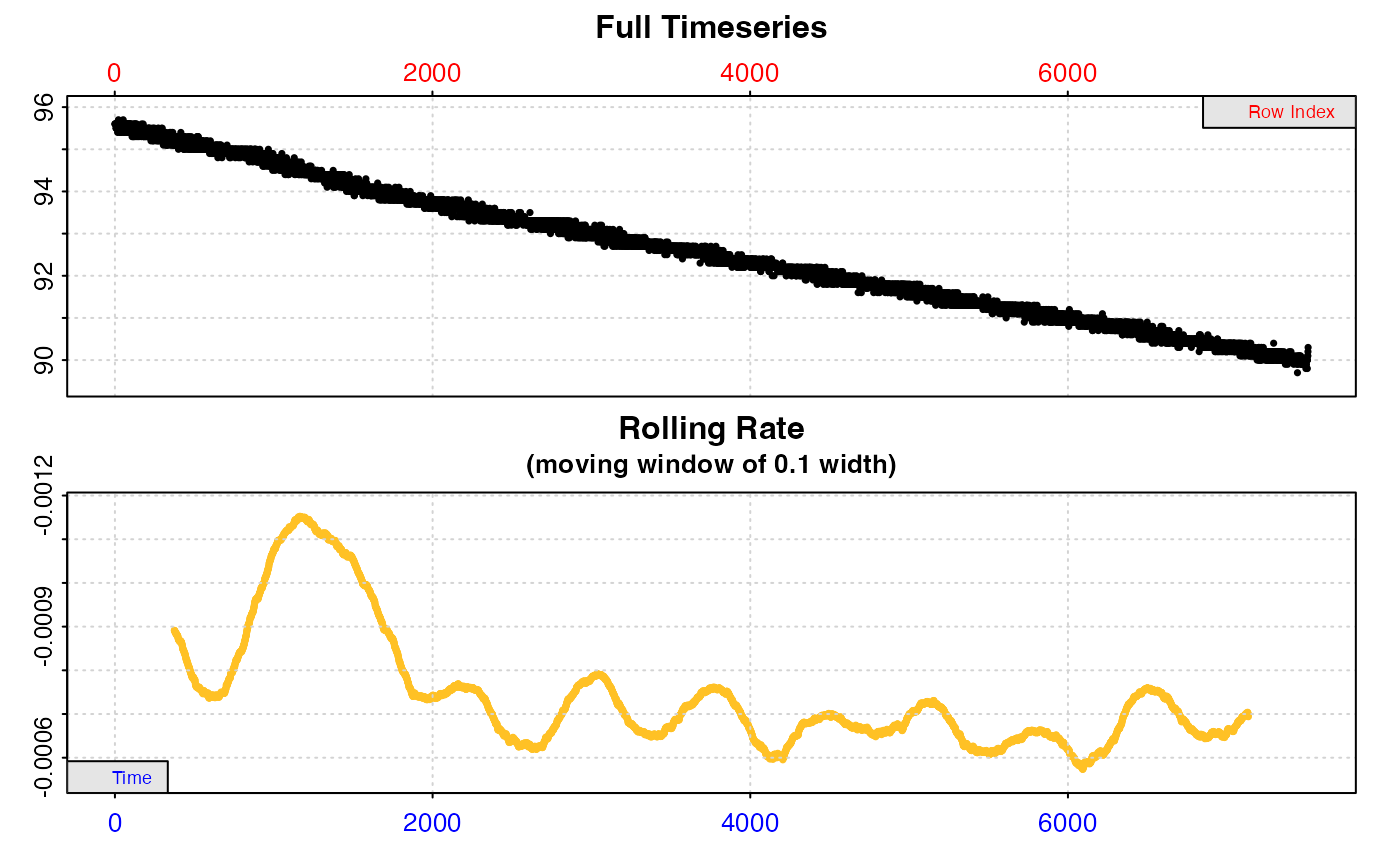
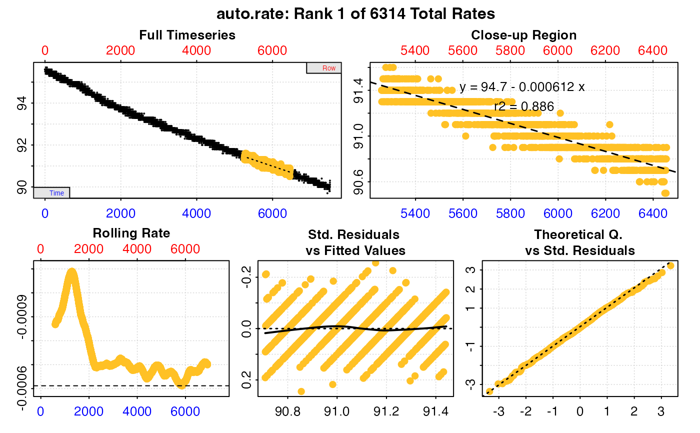
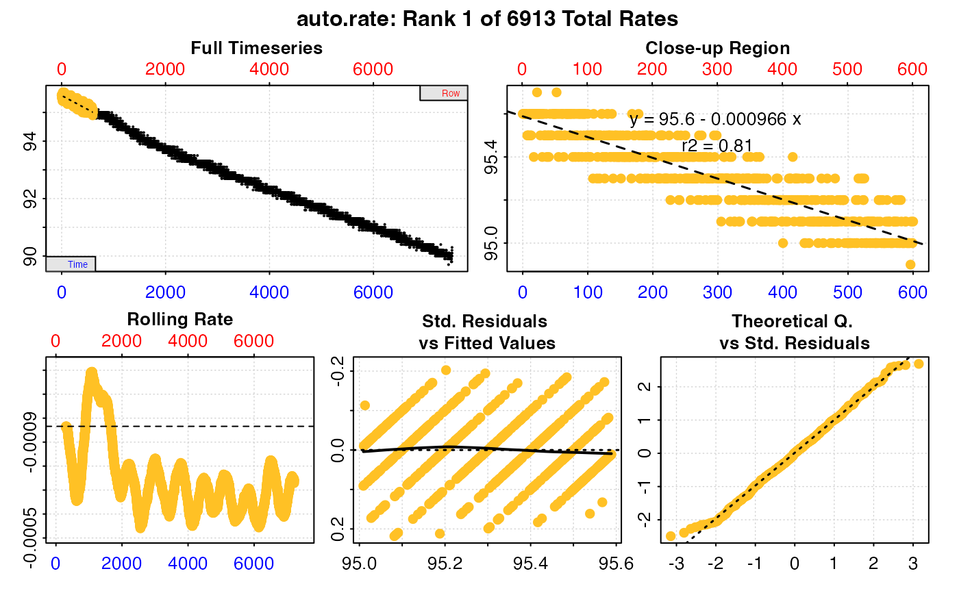
Plot
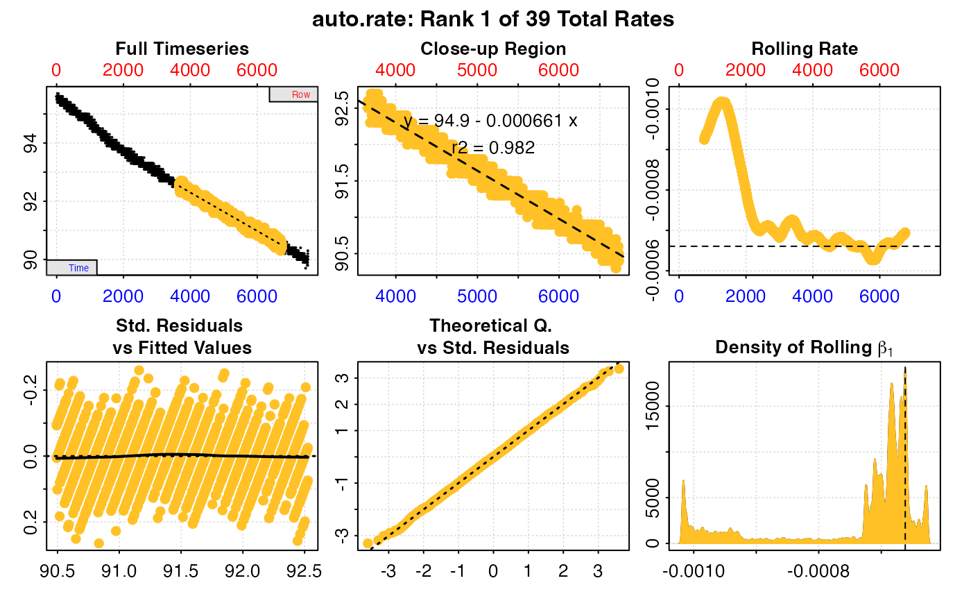
A plot is produced (provided plot = TRUE) showing the original data
timeseries of oxygen against time (bottom blue axis) and row index (top red
axis), with the rate result region highlighted. Second panel is a close-up of
the rate region with linear model coefficients. Third panel is a rolling rate
plot (note the reversed y-axis so that higher oxygen uptake rates are plotted
higher), of a rolling rate of the input width across the whole dataset.
Each rate is plotted against the middle of the time and row range used to
calculate it. The dashed line indicates the value of the current rate result
plotted in panels 1 and 2. The fourth and fifth panels are summary plots of
fit and residuals, and for the linear method the sisth panel the results of
the kernel density analysis, with the dashed line again indicating the value
of the current rate result plotted in panels 1 and 2.
Additional plotting options
If multiple rates have been calculated, by default the first (pos = 1) is
plotted. Others can be plotted by changing the pos input either in the main
function call, or by plotting the output, e.g. plot(object, pos = 2). In
addition, each sub-panel can be examined individually by using the panel
input, e.g. plot(object, panel = 2).
Console output messages can be suppressed using quiet = TRUE. If axis
labels or other text boxes obscure parts of the plot they can be suppressed
using legend = FALSE. The rate in the rolling rate plot can be plotted
not reversed by passing rate.rev = FALSE, for instance when examining
oxygen production rates so that higher production rates appear higher. If
axis labels (particularly y-axis) are difficult to read, las = 2 can be
passed to make axis labels horizontal, and oma (outer margins, default oma = c(0.4, 1, 1.5, 0.4)), and mai (inner margins, default mai = c(0.3, 0.15, 0.35, 0.15)) used to adjust plot margins.
S3 Generic Functions
Saved output objects can be used in the generic S3 functions print(),
summary(), and mean().
print(): prints a single result, by default the first rate. Others can be printed by passing theposinput. e.g.print(x, pos = 2)summary(): prints summary table of all results and metadata, or those specified by theposinput. e.g.summary(x, pos = 1:5). The summary can be exported as a separate data frame by passingexport = TRUE.mean(): calculates the mean of all rates, or those specified by theposinput. e.g.mean(x, pos = 1:5)The mean can be exported as a separate value by passingexport = TRUE.
More
For additional help, documentation, vignettes, and more visit the respR
website at https://januarharianto.github.io/respR/
Examples
# \donttest{
# Most linear section of an entire dataset
inspect(sardine.rd, time = 1, oxygen =2) %>%
auto_rate()
#> inspect: No issues detected while inspecting data frame.
#>
#> # print.inspect # -----------------------
#> Time Oxygen
#> numeric pass pass
#> Inf/-Inf pass pass
#> NA/NaN pass pass
#> sequential pass -
#> duplicated pass -
#> evenly-spaced pass -
#>
#> -----------------------------------------
 #> auto_rate: Applying default 'width' of 0.2
 #>
#> # print.auto_rate # ---------------------
#> Data extracted by 'row' using 'width' of 1502.
#> Rates computed using 'linear' method.39 linear regions detected in the kernel density estimate.
#> To see all results use summary().
#>
#> Position 1 of 39 :
#> Rate: -0.000660665
#> R.sq: 0.982
#> Rows: 3659 to 6736
#> Time: 3658 to 6735
#> -----------------------------------------
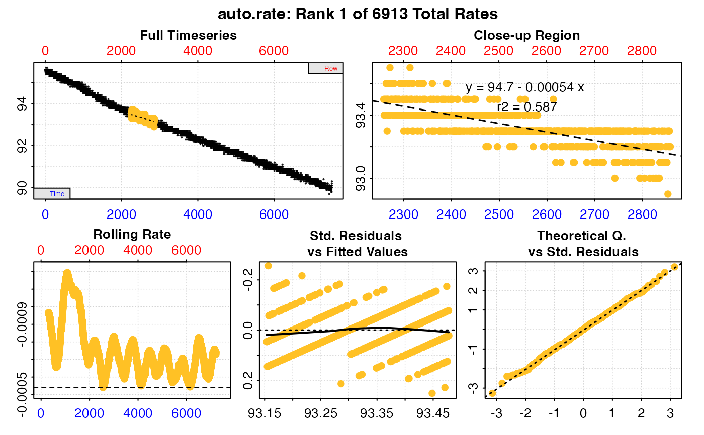
# What is the lowest oxygen consumption rate over a 10 minute (600s) period?
inspect(sardine.rd, time = 1, oxygen =2) %>%
auto_rate(method = "lowest", width = 600, by = "time") %>%
summary()
#> inspect: No issues detected while inspecting data frame.
#>
#> # print.inspect # -----------------------
#> Time Oxygen
#> numeric pass pass
#> Inf/-Inf pass pass
#> NA/NaN pass pass
#> sequential pass -
#> duplicated pass -
#> evenly-spaced pass -
#>
#> -----------------------------------------
#>
#> # print.auto_rate # ---------------------
#> Data extracted by 'row' using 'width' of 1502.
#> Rates computed using 'linear' method.39 linear regions detected in the kernel density estimate.
#> To see all results use summary().
#>
#> Position 1 of 39 :
#> Rate: -0.000660665
#> R.sq: 0.982
#> Rows: 3659 to 6736
#> Time: 3658 to 6735
#> -----------------------------------------
# What is the lowest oxygen consumption rate over a 10 minute (600s) period?
inspect(sardine.rd, time = 1, oxygen =2) %>%
auto_rate(method = "lowest", width = 600, by = "time") %>%
summary()
#> inspect: No issues detected while inspecting data frame.
#>
#> # print.inspect # -----------------------
#> Time Oxygen
#> numeric pass pass
#> Inf/-Inf pass pass
#> NA/NaN pass pass
#> sequential pass -
#> duplicated pass -
#> evenly-spaced pass -
#>
#> -----------------------------------------

 #>
#> # summary.auto_rate # -------------------
#>
#> === Summary of Results by Lowest Rate ===
#> rep rank intercept_b0 slope_b1 rsq density row endrow time endtime oxy endoxy rate
#> 1: NA 1 94.69791 -0.0005403066 0.5867958 NA 2259 2859 2258 2858 93.5 93.2 -0.0005403066
#> 2: NA 2 94.70075 -0.0005414343 0.5879174 NA 2258 2858 2257 2857 93.5 93.2 -0.0005414343
#> 3: NA 3 94.70318 -0.0005424790 0.5872572 NA 2260 2860 2259 2859 93.4 93.0 -0.0005424790
#> 4: NA 4 94.70355 -0.0005425454 0.5890225 NA 2257 2857 2256 2856 93.5 93.3 -0.0005425454
#> 5: NA 5 94.23628 -0.0005437062 0.6172363 NA 5843 6443 5842 6442 91.1 90.9 -0.0005437062
#> ---
#> 6909: NA 6909 95.90440 -0.0011924976 0.8592368 NA 794 1394 793 1393 94.9 94.2 -0.0011924976
#> 6910: NA 6910 95.90479 -0.0011924976 0.8592368 NA 796 1396 795 1395 95.0 94.3 -0.0011924976
#> 6911: NA 6911 95.90461 -0.0011925141 0.8592435 NA 795 1395 794 1394 94.9 94.3 -0.0011925141
#> 6912: NA 6912 95.90255 -0.0011926910 0.8647637 NA 774 1374 773 1373 95.0 94.2 -0.0011926910
#> 6913: NA 6913 95.90614 -0.0011938629 0.8595803 NA 791 1391 790 1390 95.0 94.2 -0.0011938629
#>
#> Regressions : 6913 | Results : 6913 | Method : lowest | Roll width : 600 | Roll type : time
#> -----------------------------------------
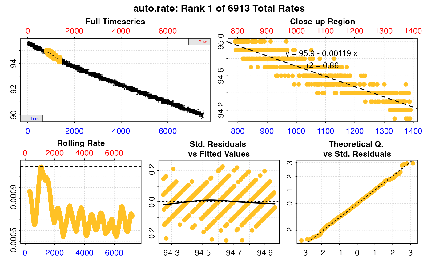
# What is the highest oxygen consumption rate over a 10 minute (600s) period?
inspect(sardine.rd, time = 1, oxygen =2) %>%
auto_rate(method = "highest", width = 600, by = "time") %>%
summary()
#> inspect: No issues detected while inspecting data frame.
#>
#> # print.inspect # -----------------------
#> Time Oxygen
#> numeric pass pass
#> Inf/-Inf pass pass
#> NA/NaN pass pass
#> sequential pass -
#> duplicated pass -
#> evenly-spaced pass -
#>
#> -----------------------------------------
#>
#> # summary.auto_rate # -------------------
#>
#> === Summary of Results by Lowest Rate ===
#> rep rank intercept_b0 slope_b1 rsq density row endrow time endtime oxy endoxy rate
#> 1: NA 1 94.69791 -0.0005403066 0.5867958 NA 2259 2859 2258 2858 93.5 93.2 -0.0005403066
#> 2: NA 2 94.70075 -0.0005414343 0.5879174 NA 2258 2858 2257 2857 93.5 93.2 -0.0005414343
#> 3: NA 3 94.70318 -0.0005424790 0.5872572 NA 2260 2860 2259 2859 93.4 93.0 -0.0005424790
#> 4: NA 4 94.70355 -0.0005425454 0.5890225 NA 2257 2857 2256 2856 93.5 93.3 -0.0005425454
#> 5: NA 5 94.23628 -0.0005437062 0.6172363 NA 5843 6443 5842 6442 91.1 90.9 -0.0005437062
#> ---
#> 6909: NA 6909 95.90440 -0.0011924976 0.8592368 NA 794 1394 793 1393 94.9 94.2 -0.0011924976
#> 6910: NA 6910 95.90479 -0.0011924976 0.8592368 NA 796 1396 795 1395 95.0 94.3 -0.0011924976
#> 6911: NA 6911 95.90461 -0.0011925141 0.8592435 NA 795 1395 794 1394 94.9 94.3 -0.0011925141
#> 6912: NA 6912 95.90255 -0.0011926910 0.8647637 NA 774 1374 773 1373 95.0 94.2 -0.0011926910
#> 6913: NA 6913 95.90614 -0.0011938629 0.8595803 NA 791 1391 790 1390 95.0 94.2 -0.0011938629
#>
#> Regressions : 6913 | Results : 6913 | Method : lowest | Roll width : 600 | Roll type : time
#> -----------------------------------------
# What is the highest oxygen consumption rate over a 10 minute (600s) period?
inspect(sardine.rd, time = 1, oxygen =2) %>%
auto_rate(method = "highest", width = 600, by = "time") %>%
summary()
#> inspect: No issues detected while inspecting data frame.
#>
#> # print.inspect # -----------------------
#> Time Oxygen
#> numeric pass pass
#> Inf/-Inf pass pass
#> NA/NaN pass pass
#> sequential pass -
#> duplicated pass -
#> evenly-spaced pass -
#>
#> -----------------------------------------

 #>
#> # summary.auto_rate # -------------------
#>
#> === Summary of Results by Highest Rate ===
#> rep rank intercept_b0 slope_b1 rsq density row endrow time endtime oxy endoxy rate
#> 1: NA 1 95.90614 -0.0011938629 0.8595803 NA 791 1391 790 1390 95.0 94.2 -0.0011938629
#> 2: NA 2 95.90255 -0.0011926910 0.8647637 NA 774 1374 773 1373 95.0 94.2 -0.0011926910
#> 3: NA 3 95.90461 -0.0011925141 0.8592435 NA 795 1395 794 1394 94.9 94.3 -0.0011925141
#> 4: NA 4 95.90479 -0.0011924976 0.8592368 NA 796 1396 795 1395 95.0 94.3 -0.0011924976
#> 5: NA 5 95.90440 -0.0011924976 0.8592368 NA 794 1394 793 1393 94.9 94.2 -0.0011924976
#> ---
#> 6909: NA 6909 94.23628 -0.0005437062 0.6172363 NA 5843 6443 5842 6442 91.1 90.9 -0.0005437062
#> 6910: NA 6910 94.70355 -0.0005425454 0.5890225 NA 2257 2857 2256 2856 93.5 93.3 -0.0005425454
#> 6911: NA 6911 94.70318 -0.0005424790 0.5872572 NA 2260 2860 2259 2859 93.4 93.0 -0.0005424790
#> 6912: NA 6912 94.70075 -0.0005414343 0.5879174 NA 2258 2858 2257 2857 93.5 93.2 -0.0005414343
#> 6913: NA 6913 94.69791 -0.0005403066 0.5867958 NA 2259 2859 2258 2858 93.5 93.2 -0.0005403066
#>
#> Regressions : 6913 | Results : 6913 | Method : highest | Roll width : 600 | Roll type : time
#> -----------------------------------------
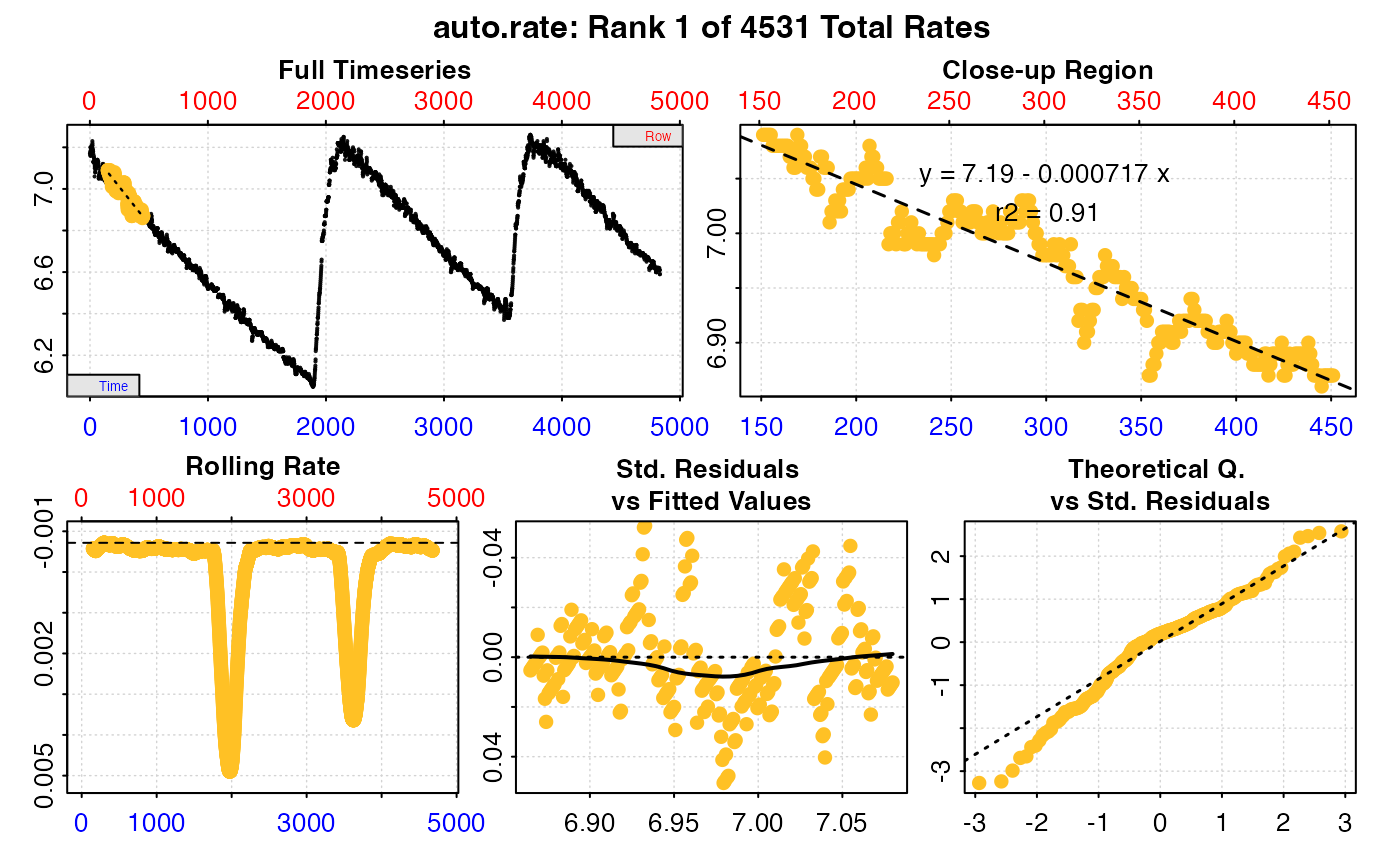
# What is the NUMERICAL minimum oxygen consumption rate over a 5 minute (300s)
# period in intermittent-flow respirometry data?
# NOTE: because uptake rates are negative, this would actually be
# the HIGHEST uptake rate.
auto_rate(intermittent.rd, method = "minimum", width = 300, by = "time") %>%
summary()
#> auto_rate: Note dataset contains both negative and positive rates. Ensure ordering 'method' is appropriate.
#>
#> # summary.auto_rate # -------------------
#>
#> === Summary of Results by Highest Rate ===
#> rep rank intercept_b0 slope_b1 rsq density row endrow time endtime oxy endoxy rate
#> 1: NA 1 95.90614 -0.0011938629 0.8595803 NA 791 1391 790 1390 95.0 94.2 -0.0011938629
#> 2: NA 2 95.90255 -0.0011926910 0.8647637 NA 774 1374 773 1373 95.0 94.2 -0.0011926910
#> 3: NA 3 95.90461 -0.0011925141 0.8592435 NA 795 1395 794 1394 94.9 94.3 -0.0011925141
#> 4: NA 4 95.90479 -0.0011924976 0.8592368 NA 796 1396 795 1395 95.0 94.3 -0.0011924976
#> 5: NA 5 95.90440 -0.0011924976 0.8592368 NA 794 1394 793 1393 94.9 94.2 -0.0011924976
#> ---
#> 6909: NA 6909 94.23628 -0.0005437062 0.6172363 NA 5843 6443 5842 6442 91.1 90.9 -0.0005437062
#> 6910: NA 6910 94.70355 -0.0005425454 0.5890225 NA 2257 2857 2256 2856 93.5 93.3 -0.0005425454
#> 6911: NA 6911 94.70318 -0.0005424790 0.5872572 NA 2260 2860 2259 2859 93.4 93.0 -0.0005424790
#> 6912: NA 6912 94.70075 -0.0005414343 0.5879174 NA 2258 2858 2257 2857 93.5 93.2 -0.0005414343
#> 6913: NA 6913 94.69791 -0.0005403066 0.5867958 NA 2259 2859 2258 2858 93.5 93.2 -0.0005403066
#>
#> Regressions : 6913 | Results : 6913 | Method : highest | Roll width : 600 | Roll type : time
#> -----------------------------------------
# What is the NUMERICAL minimum oxygen consumption rate over a 5 minute (300s)
# period in intermittent-flow respirometry data?
# NOTE: because uptake rates are negative, this would actually be
# the HIGHEST uptake rate.
auto_rate(intermittent.rd, method = "minimum", width = 300, by = "time") %>%
summary()
#> auto_rate: Note dataset contains both negative and positive rates. Ensure ordering 'method' is appropriate.
 #>
#> # summary.auto_rate # -------------------
#>
#> === Summary of Results by Minimum Rate ===
#> rep rank intercept_b0 slope_b1 rsq density row endrow time endtime oxy endoxy rate
#> 1: NA 1 7.188147 -0.0007172339 0.9100089 NA 152 452 151 451 7.09 6.87 -0.0007172339
#> 2: NA 2 7.187775 -0.0007169567 0.9095930 NA 156 456 155 455 7.09 6.84 -0.0007169567
#> 3: NA 3 7.187642 -0.0007167851 0.9095981 NA 157 457 156 456 7.08 6.85 -0.0007167851
#> 4: NA 4 7.187706 -0.0007163583 0.9096754 NA 155 455 154 454 7.09 6.84 -0.0007163583
#> 5: NA 5 7.187809 -0.0007161603 0.9098124 NA 153 453 152 452 7.09 6.87 -0.0007161603
#> ---
#> 4527: NA 4527 -3.013661 0.0048978592 0.9352893 NA 1823 2123 1822 2122 6.12 7.19 0.0048978592
#> 4528: NA 4528 -3.015906 0.0048982993 0.9353444 NA 1824 2124 1823 2123 6.11 7.18 0.0048982993
#> 4529: NA 4529 -3.020091 0.0048990913 0.9354343 NA 1826 2126 1825 2125 6.11 7.21 0.0048990913
#> 4530: NA 4530 -3.022963 0.0048992849 0.9354567 NA 1828 2128 1827 2127 6.10 7.21 0.0048992849
#> 4531: NA 4531 -3.022005 0.0048994302 0.9354734 NA 1827 2127 1826 2126 6.11 7.21 0.0048994302
#>
#> Regressions : 4531 | Results : 4531 | Method : minimum | Roll width : 300 | Roll type : time
#> -----------------------------------------
# What is the NUMERICAL maximum oxygen consumption rate over a 20 minute
# (1200 rows) period in respirometry data in which oxygen is declining?
# NOTE: because uptake rates are negative, this would actually be
# the LOWEST uptake rate.
sardine.rd %>%
inspect() %>%
auto_rate(method = "maximum", width = 1200, by = "row") %>%
summary()
#> inspect: Applying column default of 'time = 1'
#> inspect: Applying column default of 'oxygen = 2'
#> inspect: No issues detected while inspecting data frame.
#>
#> # print.inspect # -----------------------
#> Time Oxygen
#> numeric pass pass
#> Inf/-Inf pass pass
#> NA/NaN pass pass
#> sequential pass -
#> duplicated pass -
#> evenly-spaced pass -
#>
#> -----------------------------------------
#>
#> # summary.auto_rate # -------------------
#>
#> === Summary of Results by Minimum Rate ===
#> rep rank intercept_b0 slope_b1 rsq density row endrow time endtime oxy endoxy rate
#> 1: NA 1 7.188147 -0.0007172339 0.9100089 NA 152 452 151 451 7.09 6.87 -0.0007172339
#> 2: NA 2 7.187775 -0.0007169567 0.9095930 NA 156 456 155 455 7.09 6.84 -0.0007169567
#> 3: NA 3 7.187642 -0.0007167851 0.9095981 NA 157 457 156 456 7.08 6.85 -0.0007167851
#> 4: NA 4 7.187706 -0.0007163583 0.9096754 NA 155 455 154 454 7.09 6.84 -0.0007163583
#> 5: NA 5 7.187809 -0.0007161603 0.9098124 NA 153 453 152 452 7.09 6.87 -0.0007161603
#> ---
#> 4527: NA 4527 -3.013661 0.0048978592 0.9352893 NA 1823 2123 1822 2122 6.12 7.19 0.0048978592
#> 4528: NA 4528 -3.015906 0.0048982993 0.9353444 NA 1824 2124 1823 2123 6.11 7.18 0.0048982993
#> 4529: NA 4529 -3.020091 0.0048990913 0.9354343 NA 1826 2126 1825 2125 6.11 7.21 0.0048990913
#> 4530: NA 4530 -3.022963 0.0048992849 0.9354567 NA 1828 2128 1827 2127 6.10 7.21 0.0048992849
#> 4531: NA 4531 -3.022005 0.0048994302 0.9354734 NA 1827 2127 1826 2126 6.11 7.21 0.0048994302
#>
#> Regressions : 4531 | Results : 4531 | Method : minimum | Roll width : 300 | Roll type : time
#> -----------------------------------------
# What is the NUMERICAL maximum oxygen consumption rate over a 20 minute
# (1200 rows) period in respirometry data in which oxygen is declining?
# NOTE: because uptake rates are negative, this would actually be
# the LOWEST uptake rate.
sardine.rd %>%
inspect() %>%
auto_rate(method = "maximum", width = 1200, by = "row") %>%
summary()
#> inspect: Applying column default of 'time = 1'
#> inspect: Applying column default of 'oxygen = 2'
#> inspect: No issues detected while inspecting data frame.
#>
#> # print.inspect # -----------------------
#> Time Oxygen
#> numeric pass pass
#> Inf/-Inf pass pass
#> NA/NaN pass pass
#> sequential pass -
#> duplicated pass -
#> evenly-spaced pass -
#>
#> -----------------------------------------
 #>
#> # summary.auto_rate # -------------------
#>
#> === Summary of Results by Maximum Rate ===
#> rep rank intercept_b0 slope_b1 rsq density row endrow time endtime oxy endoxy rate
#> 1: NA 1 94.65936 -0.0006119306 0.8860806 NA 5258 6457 5257 6456 91.4 90.9 -0.0006119306
#> 2: NA 2 94.66030 -0.0006121060 0.8873339 NA 5255 6454 5254 6453 91.5 90.7 -0.0006121060
#> 3: NA 3 94.66062 -0.0006121414 0.8861755 NA 5259 6458 5258 6457 91.3 90.7 -0.0006121414
#> 4: NA 4 94.66144 -0.0006122921 0.8873521 NA 5254 6453 5253 6452 91.5 90.8 -0.0006122921
#> 5: NA 5 94.66291 -0.0006124744 0.8881668 NA 5245 6444 5244 6443 91.5 90.6 -0.0006124744
#> ---
#> 6310: NA 6310 95.78939 -0.0010891497 0.9541232 NA 693 1892 692 1891 95.0 93.8 -0.0010891497
#> 6311: NA 6311 95.78963 -0.0010892612 0.9541131 NA 695 1894 694 1893 95.0 93.8 -0.0010892612
#> 6312: NA 6312 95.78948 -0.0010892893 0.9541535 NA 692 1891 691 1890 95.0 93.8 -0.0010892893
#> 6313: NA 6313 95.78974 -0.0010894181 0.9541472 NA 694 1893 693 1892 95.0 93.7 -0.0010894181
#> 6314: NA 6314 95.78956 -0.0010894205 0.9541820 NA 691 1890 690 1889 95.0 93.7 -0.0010894205
#>
#> Regressions : 6314 | Results : 6314 | Method : maximum | Roll width : 1200 | Roll type : row
#> -----------------------------------------
# Perform a rolling regression of 10 minutes width across the entire dataset.
# Results are not ordered under this method.
sardine.rd %>%
inspect() %>%
auto_rate(method = "rolling", width = 600, by = "time") %>%
summary()
#> inspect: Applying column default of 'time = 1'
#> inspect: Applying column default of 'oxygen = 2'
#> inspect: No issues detected while inspecting data frame.
#>
#> # print.inspect # -----------------------
#> Time Oxygen
#> numeric pass pass
#> Inf/-Inf pass pass
#> NA/NaN pass pass
#> sequential pass -
#> duplicated pass -
#> evenly-spaced pass -
#>
#> -----------------------------------------
#>
#> # summary.auto_rate # -------------------
#>
#> === Summary of Results by Maximum Rate ===
#> rep rank intercept_b0 slope_b1 rsq density row endrow time endtime oxy endoxy rate
#> 1: NA 1 94.65936 -0.0006119306 0.8860806 NA 5258 6457 5257 6456 91.4 90.9 -0.0006119306
#> 2: NA 2 94.66030 -0.0006121060 0.8873339 NA 5255 6454 5254 6453 91.5 90.7 -0.0006121060
#> 3: NA 3 94.66062 -0.0006121414 0.8861755 NA 5259 6458 5258 6457 91.3 90.7 -0.0006121414
#> 4: NA 4 94.66144 -0.0006122921 0.8873521 NA 5254 6453 5253 6452 91.5 90.8 -0.0006122921
#> 5: NA 5 94.66291 -0.0006124744 0.8881668 NA 5245 6444 5244 6443 91.5 90.6 -0.0006124744
#> ---
#> 6310: NA 6310 95.78939 -0.0010891497 0.9541232 NA 693 1892 692 1891 95.0 93.8 -0.0010891497
#> 6311: NA 6311 95.78963 -0.0010892612 0.9541131 NA 695 1894 694 1893 95.0 93.8 -0.0010892612
#> 6312: NA 6312 95.78948 -0.0010892893 0.9541535 NA 692 1891 691 1890 95.0 93.8 -0.0010892893
#> 6313: NA 6313 95.78974 -0.0010894181 0.9541472 NA 694 1893 693 1892 95.0 93.7 -0.0010894181
#> 6314: NA 6314 95.78956 -0.0010894205 0.9541820 NA 691 1890 690 1889 95.0 93.7 -0.0010894205
#>
#> Regressions : 6314 | Results : 6314 | Method : maximum | Roll width : 1200 | Roll type : row
#> -----------------------------------------
# Perform a rolling regression of 10 minutes width across the entire dataset.
# Results are not ordered under this method.
sardine.rd %>%
inspect() %>%
auto_rate(method = "rolling", width = 600, by = "time") %>%
summary()
#> inspect: Applying column default of 'time = 1'
#> inspect: Applying column default of 'oxygen = 2'
#> inspect: No issues detected while inspecting data frame.
#>
#> # print.inspect # -----------------------
#> Time Oxygen
#> numeric pass pass
#> Inf/-Inf pass pass
#> NA/NaN pass pass
#> sequential pass -
#> duplicated pass -
#> evenly-spaced pass -
#>
#> -----------------------------------------

 #>
#> # summary.auto_rate # -------------------
#>
#> === Summary of Results by Rolling Order ===
#> rep rank intercept_b0 slope_b1 rsq density row endrow time endtime oxy endoxy rate
#> 1: NA 1 95.58876 -0.0009658708 0.8098300 NA 1 601 0 600 95.6 95.1 -0.0009658708
#> 2: NA 2 95.58805 -0.0009625044 0.8073351 NA 2 602 1 601 95.6 95.2 -0.0009625044
#> 3: NA 3 95.58799 -0.0009624325 0.8073155 NA 3 603 2 602 95.6 95.0 -0.0009624325
#> 4: NA 4 95.58792 -0.0009623275 0.8072869 NA 4 604 3 603 95.6 95.0 -0.0009623275
#> 5: NA 5 95.58751 -0.0009605309 0.8063767 NA 5 605 4 604 95.6 95.1 -0.0009605309
#> ---
#> 6909: NA 6909 95.52650 -0.0007437493 0.7536903 NA 6909 7509 6908 7508 90.4 90.0 -0.0007437493
#> 6910: NA 6910 95.50646 -0.0007409356 0.7508723 NA 6910 7510 6909 7509 90.4 90.1 -0.0007409356
#> 6911: NA 6911 95.48630 -0.0007381054 0.7480377 NA 6911 7511 6910 7510 90.3 90.1 -0.0007381054
#> 6912: NA 6912 95.46638 -0.0007352640 0.7432546 NA 6912 7512 6911 7511 90.4 90.2 -0.0007352640
#> 6913: NA 6913 95.42246 -0.0007290949 0.7329032 NA 6913 7513 6912 7512 90.4 90.3 -0.0007290949
#>
#> Regressions : 6913 | Results : 6913 | Method : rolling | Roll width : 600 | Roll type : time
#> -----------------------------------------
# }
#>
#> # summary.auto_rate # -------------------
#>
#> === Summary of Results by Rolling Order ===
#> rep rank intercept_b0 slope_b1 rsq density row endrow time endtime oxy endoxy rate
#> 1: NA 1 95.58876 -0.0009658708 0.8098300 NA 1 601 0 600 95.6 95.1 -0.0009658708
#> 2: NA 2 95.58805 -0.0009625044 0.8073351 NA 2 602 1 601 95.6 95.2 -0.0009625044
#> 3: NA 3 95.58799 -0.0009624325 0.8073155 NA 3 603 2 602 95.6 95.0 -0.0009624325
#> 4: NA 4 95.58792 -0.0009623275 0.8072869 NA 4 604 3 603 95.6 95.0 -0.0009623275
#> 5: NA 5 95.58751 -0.0009605309 0.8063767 NA 5 605 4 604 95.6 95.1 -0.0009605309
#> ---
#> 6909: NA 6909 95.52650 -0.0007437493 0.7536903 NA 6909 7509 6908 7508 90.4 90.0 -0.0007437493
#> 6910: NA 6910 95.50646 -0.0007409356 0.7508723 NA 6910 7510 6909 7509 90.4 90.1 -0.0007409356
#> 6911: NA 6911 95.48630 -0.0007381054 0.7480377 NA 6911 7511 6910 7510 90.3 90.1 -0.0007381054
#> 6912: NA 6912 95.46638 -0.0007352640 0.7432546 NA 6912 7512 6911 7511 90.4 90.2 -0.0007352640
#> 6913: NA 6913 95.42246 -0.0007290949 0.7329032 NA 6913 7513 6912 7512 90.4 90.3 -0.0007290949
#>
#> Regressions : 6913 | Results : 6913 | Method : rolling | Roll width : 600 | Roll type : time
#> -----------------------------------------
# }