Oxygen production respirometry

Introduction

While the majority of respirometry studies are concerned with oxygen uptake by various organisms, there are many studies of organisms such as plants, algae and corals where oxygen production rates are of primary interest. We have designed respR to be able to process and calculate rates from oxygen production data in exactly the same way as for consumption data. In fact, the package has already been used by several studies to determine the production rates of diatoms, algae, and corals.

Here we will use the included algae.rd dataset to briefly show how production data may be processed and used to extract production rates. It contains 20 hours of data recorded once per minute on oxygen production by an algae. More information on the data can be seen by running ?algae.rd.

Inspect the data

Like all analyses in respR the first step is to inspect the data for common issues.

inspect(algae.rd, rate.rev = FALSE)
#> inspect: Applying column default of 'time = 1'
#> inspect: Applying column default of 'oxygen = 2'
#> Warning: inspect: Time values are not evenly-spaced (numerically).
#> inspect: Data issues detected. For more information use print().
#> 
#> # print.inspect # -----------------------
#>                 Time Oxygen
#> numeric         pass   pass
#> Inf/-Inf        pass   pass
#> NA/NaN          pass   pass
#> sequential      pass      -
#> duplicated      pass      -
#> evenly-spaced   WARN      -
#> 
#> Uneven Time data locations (first 20 shown) in column: Time 
#>  [1]  1  2  3  4  5  6  7  8  9 10 11 12 13 14 15 16 17 18 19 20
#> Minimum and Maximum intervals in uneven Time data: 
#> [1] 0.01 0.02
#> -----------------------------------------

In respR oxygen uptake rates are represented by negative values since they represent a negative slope of oxygen against time. Since the focus of the package is on uptake rates, by default the inspect() function plots rolling rates on a reversed axis so that higher oxygen uptake rates appear higher on the plot. To examine production rates, which are positive, we pass rate.rev = FALSE to reverse this behaviour

We can see the data passes most of the checks. The warning about uneven time can be safely disregarded as it stems from the per minute recording interval being converted to decimalised hours, and we can see the minimum and maximum intervals indicate there are no major gaps.

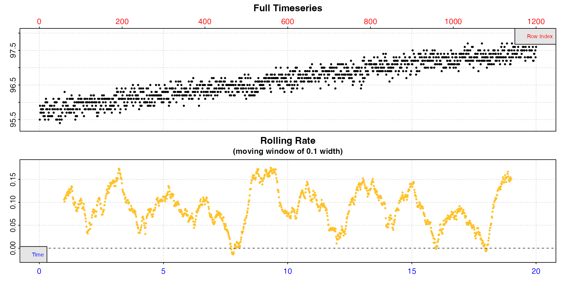
We can see that at the default rolling rate width input of 10% of the data the rate is very variable, from zero to over 0.15. However, there are characteristics of the raw data which could cause this; it has a fairly shallow overall slope and high relative noise level, therefore rates over narrow time windows would be expected to be variable. Instead we can pick a more appropriate width that will give a better idea of the true rate.

algae_insp <- inspect(algae.rd, width = 0.5, rate.rev = FALSE)
#> inspect: Applying column default of 'time = 1'
#> inspect: Applying column default of 'oxygen = 2'
#> Warning: inspect: Time values are not evenly-spaced (numerically).
#> inspect: Data issues detected. For more information use print().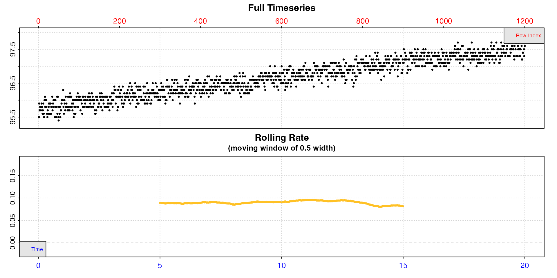

We can see now that rate is actually highly stable across the dataset, and this tells us when we come to calculate rates we should probably use rates determined over this width or higher, and the value will be around 0.09 to 0.10.

Calculate rates

Since the rate appears to be fairly stable across the dataset we will use auto_rate() to identify the most linear region.

algae_rate <- auto_rate(algae_insp, rate.rev = FALSE) 
#> auto_rate: Applying default 'width' of 0.2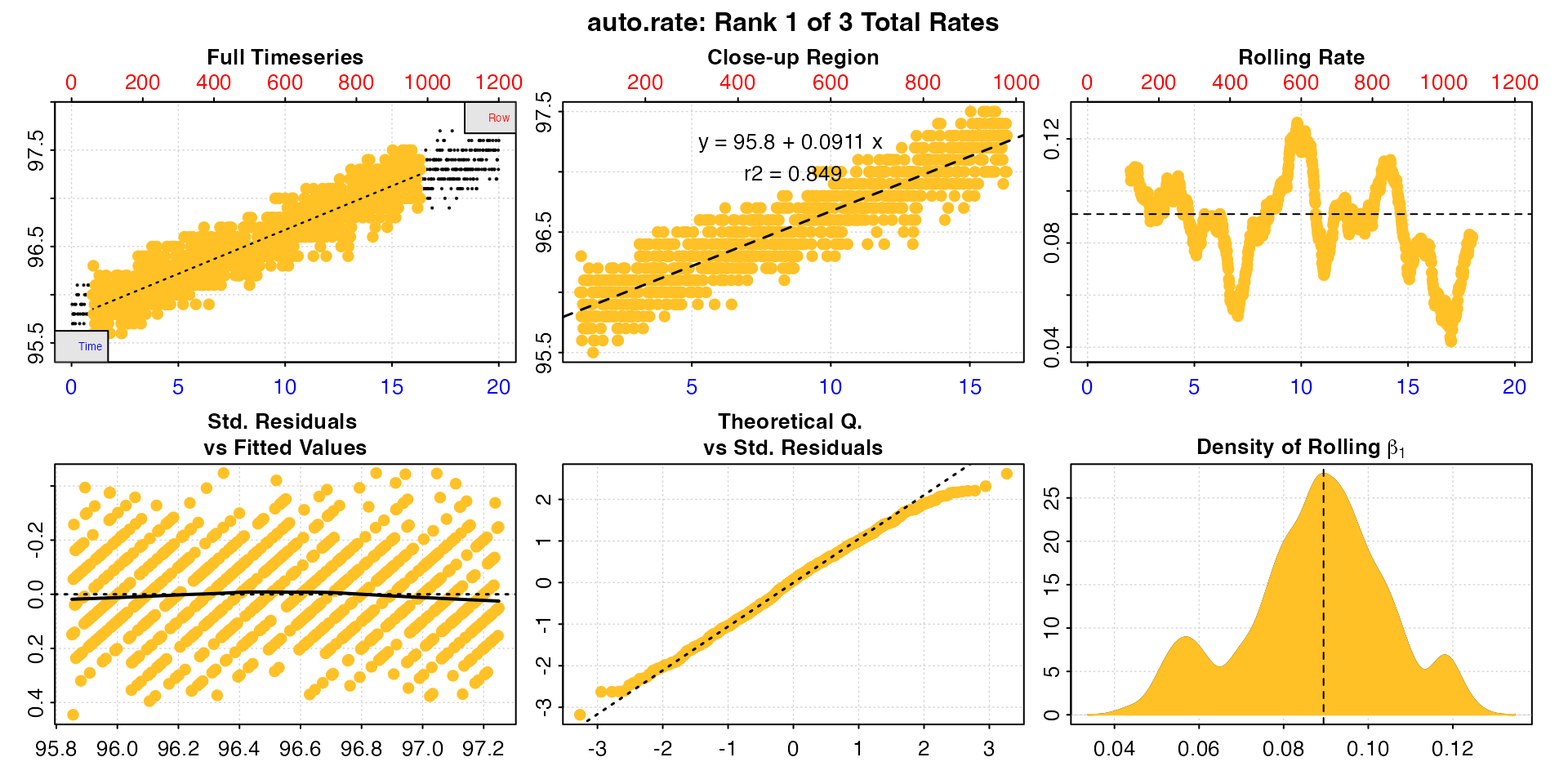

This is a good opportunity to explain how the auto_rate "linear" method works and how to interpret the outputs. Briefly (see vignette("auto_rate") for more detail), the linear method uses the input width as a starting seed value to calculate a rolling rate across the dataset (seen in panel 3). It then uses these rates to identify linear regions using kernel density estimation (KDE, see panel 6). Peaks in this plot represent linear regions, that is areas of stable rates at that width representative of that region as a whole. It then re-samples these regions and runs additional linear analysis at different widths to arrive at a final rate for this region. This is why the final, high ranked rates tend to be over widths greater than the input width, as can be seen here with the top ranked result.

summary(algae_rate)
#> 
#> # summary.auto_rate # -------------------
#> 
#> === Summary of Results by Kernel Density Rank ===
#>    rep rank intercept_b0 slope_b1   rsq density row endrow  time endtime  oxy endoxy   rate
#> 1:  NA    1         95.8   0.0911 0.849   27.76  59    980  0.98    16.3 96.0   97.3 0.0911
#> 2:  NA    2         96.4   0.0507 0.128    8.92 891   1144 14.85    19.1 97.1   97.3 0.0507
#> 3:  NA    3         95.5   0.1194 0.441    6.86 460    714  7.67    11.9 96.2   96.6 0.1194
#> 
#> Regressions : 961 | Results : 3 | Method : linear | Roll width : 240 | Roll type : row 
#> -----------------------------------------

Here, we have a very good top ranked result; it is calculated over a large part of the dataset, is around the value we expected from inspecting it earlier, this value is in the middle of the range of rolling rates at the default input width (dashed line, panel 3), and has a high r-squared in comparison to the other results.

Generally, the higher and wider the peak in the KDE, the more linear the region. We can see three peaks in the KDE (panel 6). However, the other two are very much lower and narrower. Let’s look at the second ranked result using pos.

plot(algae_rate, pos = 2, rate.rev = FALSE)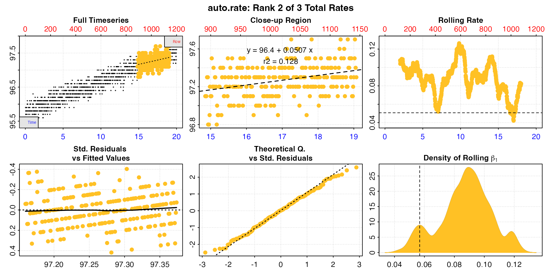

Here we can see this rate is over a much narrower region towards the end of the data, the value of 0.05 is very much lower than we are expecting, and at the extremes of the range (panel 3). While this may be a linear region within the data, it is very much not representative of the data as a whole.

In this analysis, we can easily see that the top ranked result is the one we want, and we can exclude the other two. See vignette("select_rate") for more advanced filtering of auto_rate results by many different criteria.

Rolling rate widths in `auto_rate`

We saw in the inspect section above a higher width made the rolling rate much more consistent. It is not necessarily always the case increasing the default of width = 0.2 will improve the results of auto_rate however, as it gives the KDE much less variation to work with.

Here is the summary table of the results when we increase the width to 0.5. Note that the rolling rate plot (panel 3) in which the rate looks highly variable is now on a much narrower y-axis range. In fact, it is identical to the one in the inspect plot above but on different axes ranges.

auto_rate(algae_insp, width = 0.5, rate.rev = FALSE)$summary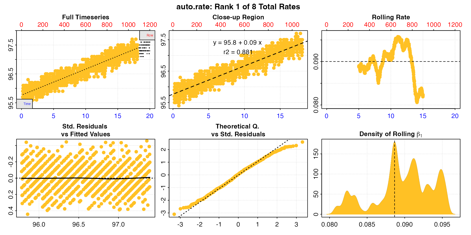

#>      rep  rank intercept_b0 slope_b1   rsq density   row endrow  time endtime   oxy endoxy   rate
#>    <num> <int>        <num>    <num> <num>   <num> <int>  <int> <num>   <num> <num>  <num>  <num>
#> 1:    NA     1         95.8   0.0900 0.881   179.4    11   1086  0.18    18.1  95.7   97.2 0.0900
#> 2:    NA     2         95.8   0.0899 0.855   138.3   132   1083  2.20    18.1  96.2   97.3 0.0899
#> 3:    NA     3         95.7   0.0916 0.761   111.2   338   1016  5.63    16.9  96.2   97.3 0.0916
#> 4:    NA     4         95.8   0.0910 0.763    74.3   328   1016  5.47    16.9  96.3   97.3 0.0910
#> 5:    NA     5         95.9   0.0813 0.651    57.9   612   1200 10.20    20.0  96.9   97.6 0.0813
#> 6:    NA     6         95.9   0.0820 0.651    46.8   612   1192 10.20    19.9  96.9   97.6 0.0820
#> 7:    NA     7         95.8   0.0903 0.824    27.4   203   1042  3.38    17.4  96.3   97.2 0.0903
#> 8:    NA     8         95.8   0.0852 0.639    20.1   543   1083  9.05    18.1  96.7   97.3 0.0852

This doesn’t really improve our analysis very much, and could be more confusing since there are more results. There is still one central peak in the KDE analysis, which uses more of the dataset, but it is largely the same as the top ranked result in the earlier analysis, differing in rate value by only 1-2%. The other results are more consistent in their rate values, but they are largely redundant as they broadly use the same range of the data. We can visualise this using the internal overlap.p() function.

auto_rate(algae_insp, width = 0.5, rate.rev = FALSE, plot = FALSE) |>
  respR:::overlap.p()
#> overlap.p: Plotting all rate(s)...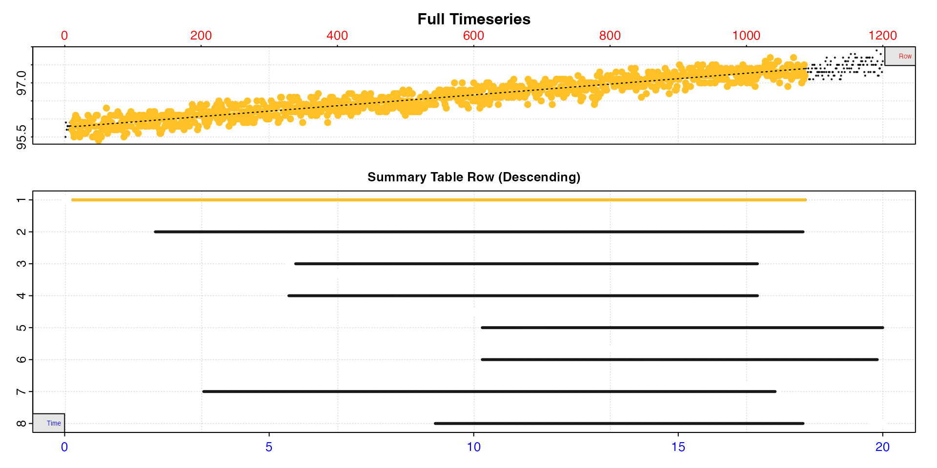

So we could use the top ranked result here, but the ultimate rate value barely differs from our earlier analysis, and in this case the default width provided us with a valid result, so there is no real reason to exclude it. This does however serve as a good example of how users should experiment with different widths in auto_rate to get an idea of how it might affect analyses. Certain datasets will benefit from this more than others.

See Prinzing et al. 2021 for an excellent discussion of appropriate widths in rolling regressions to determine maximum metabolic rates, much of which is relevant to extracting rates of any kind.

Adjust rate

Oxygen production rates can be adjusted in the exact same way as uptake rates. In most oxygen production respirometry, background is likely similar to that in uptake respirometry, that is microbial organisms are consuming oxygen. However there may be cases where some of the production could be contributed by other organisms, such as another algae growing on the surfaces of the respirometer. What is important is to quantify this by running blank experiments which are identical in every way except for the presence of the specimen you are interested in. See vignette("adjust_rate") for details of the numerous ways experiments can be background adjusted, most of which is equally relevant to oxygen production respirometry.

Here, we don’t have a control experiment to work with, so we will just invent some values. The most important aspect here is to be careful with the signs of the rates we are using; production rates are positive, uptake rates negative.

This is how you would adjust for a oxygen uptake by micro-organisms. The uptake background is negative, which means the production rates have been under-estimated.

algae_rate_adj <- adjust_rate(algae_rate, by = -0.007)  
#> adjust_rate: Rate adjustments applied using "mean" method.
summary(algae_rate_adj)
#> 
#> # summary.adjust_rate # -----------------
#> 
#> Adjustment was applied using 'mean' method.
#> Summary of all rate results:
#> 
#>    rep rank intercept_b0 slope_b1   rsq density row endrow  time endtime  oxy endoxy   rate adjustment rate.adjusted
#> 1:  NA    1         95.8   0.0911 0.849   27.76  59    980  0.98    16.3 96.0   97.3 0.0911     -0.007        0.0981
#> 2:  NA    2         96.4   0.0507 0.128    8.92 891   1144 14.85    19.1 97.1   97.3 0.0507     -0.007        0.0577
#> 3:  NA    3         95.5   0.1194 0.441    6.86 460    714  7.67    11.9 96.2   96.6 0.1194     -0.007        0.1264
#> -----------------------------------------

If however you find the control has a background input of oxygen it is entered as a positive value, in which case the specimen production rates have been over-estimated.

adjust_rate(algae_rate, by = 0.009) |>
  summary()
#> adjust_rate: Rate adjustments applied using "mean" method.
#> 
#> # summary.adjust_rate # -----------------
#> 
#> Adjustment was applied using 'mean' method.
#> Summary of all rate results:
#> 
#>    rep rank intercept_b0 slope_b1   rsq density row endrow  time endtime  oxy endoxy   rate adjustment rate.adjusted
#> 1:  NA    1         95.8   0.0911 0.849   27.76  59    980  0.98    16.3 96.0   97.3 0.0911      0.009        0.0821
#> 2:  NA    2         96.4   0.0507 0.128    8.92 891   1144 14.85    19.1 97.1   97.3 0.0507      0.009        0.0417
#> 3:  NA    3         95.5   0.1194 0.441    6.86 460    714  7.67    11.9 96.2   96.6 0.1194      0.009        0.1104
#> -----------------------------------------

See also Case 9 in vignette("adjust_rate") where we perform a similar adjustment to production rates.

Convert rate

Production rates are converted to units in exactly the same way as uptake rates.

New in respR v2.0 is the ability to output rates as surface-area specific, which is often used to express oxygen production of algae and corals per unit area, so we’ll add an area input and specify an area-specific output.unit.

The area input must be in units of $m^2$ . Here we can also use the new convert_val() function to enter the area input. This function converts between units of area, mass, etc. It is particularly handy in convert_rate because the default output unit for area conversions is $m^2$ . Let’s say our algae is 10 $cm^2$ . We don’t have to do this conversion ourselves, but can rely on convert_val. We don’t even need to tell it this is an area conversion - it detects this automatically from the input units.

algae_rate_conv <- convert_rate(algae_rate_adj, 
                                oxy.unit = "%Air", 
                                time.unit = "hr", 
                                output.unit = "mg/h/m2",
                                area = convert_val(10, "cm2"),
                                volume = 0.1,
                                t = 12, S = 30, P =1.01)
#> convert_rate: Object of class 'adjust_rate' detected. Converting all adjusted rates in '$rate.adjusted'.

In this case, we were only interested in the top ranked rate result. We can extract it using summary and the pos and export inputs. We can see the converted area input in $m^2$ in the summary table.

summary(algae_rate_conv, pos = 1, export = TRUE)
#> 
#> # summary.convert_rate # ----------------
#> Summary of converted rates from entered 'pos' rank(s):
#> 
#>    rep rank intercept_b0 slope_b1   rsq density row endrow time endtime oxy endoxy   rate adjustment rate.adjusted rate.input oxy.unit time.unit volume mass  area  S  t    P rate.abs rate.m.spec rate.a.spec output.unit rate.output
#> 1:  NA    1         95.8   0.0911 0.849    27.8  59    980 0.98    16.3  96   97.3 0.0911     -0.007        0.0981     0.0981     %Air        hr    0.1   NA 0.001 30 12 1.01 0.000872          NA       0.872  mgO2/hr/m2       0.872
#> -----------------------------------------