calc_rate.int: Manual extraction of rates in intermittent-flow respirometry

Introduction

calc_rate.int() is a function for manually determining rates across user-defined ranges of row or time in each replicate in intermittent-flow respirometry data. This page contains descriptions and simple examples of the functionality. See also the help file at help("calc_rate.int"), see vignette("intermittent_short") for how it can be used to analyse a relatively brief intermittent-flow respirometry experiment, and vignette("intermittent_long") for an example of analysing a longer experiment.

Overview

How calc_rate.int works is fairly straightforward. The function uses the starts locations to subset each replicate from the data in x. It extracts a rate using the wait and measure inputs in the by metric.

A calc_rate object is saved for each replicate in the output in $results, and the output $summary table contains the results from all replicates in order with the $rep column indicating the replicate number. This output object can be passed to subsequent functions such as adjust_rate() and convert_rate() for further processing.

Inputs

There are two required inputs:

x: The time~oxygen data from a single intermittent-flow experiment as either a data.frame or an inspect object
starts: The location of the start of each replicate. This can be either:
- A numeric vector of row numbers or times indicating each replicate start location.
- A single numeric value representing a regular row or time interval starting from the first row or time value in the data. This option should only be used when replicates cycle at regular intervals. If the first replicate does not start at row 1 of the data in x it should be subset so that it does. See subset_data() and examples below for how to do this.

Other inputs

wait: Rows or time period to exclude at the start of each replicate.
measure: Rows or time period over which to calculate rate in each replicate. Applied directly after wait phase.
by: Method by which starts, wait and measure are applied. Either "row" or "time".
plot: Controls if a plot is produced. See Plot section.

Irregularly spaced replicates

Data

The urchin dataset used for examples below is the included intermittent.rd example data with the time values changed to minutes to better demonstrate time region selection. Experimental data such as volume, weight, and row locations of replicates, flushes etc. can be found in the data help file: ?intermittent.rd.

urchin <- intermittent.rd
urchin[[1]] <- round(urchin[[1]] / 60, 2) # change time values to minutes and round them

This is what the whole dataset look like. There are three replicates, and note they are of different duration.

urchin <- inspect(urchin)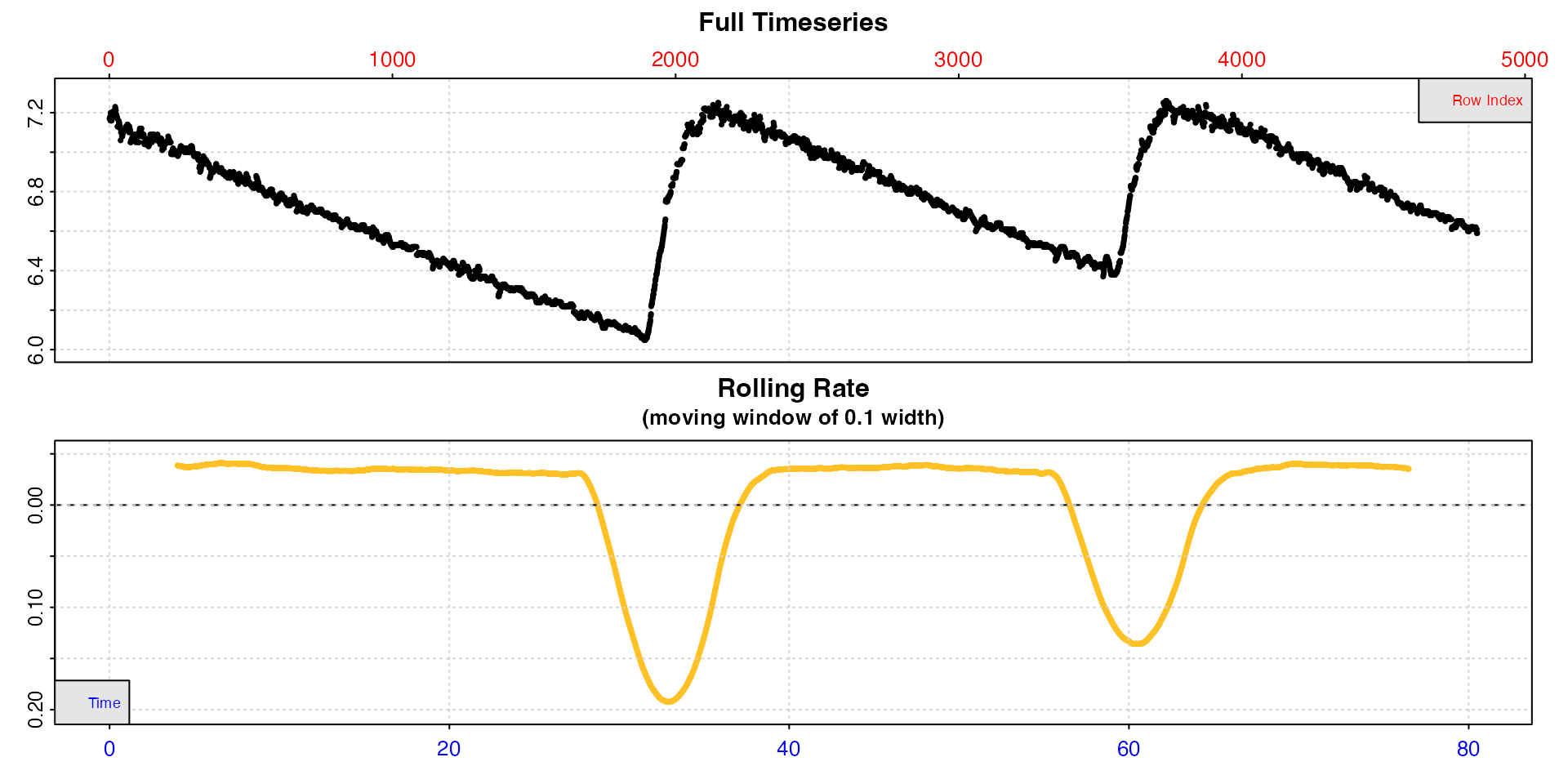

Rate from `row` range in each replicate

If no inputs other than x and starts (in the default units of by = "row") are entered, the default behaviour is to calculate a rate across all the data in each replicate.

calc_rate.int(urchin,
              starts = c(1, 2101, 3901)) 
#> calc_rate.int: The `measure` input is NULL. Calculating rate to the end of the replicate.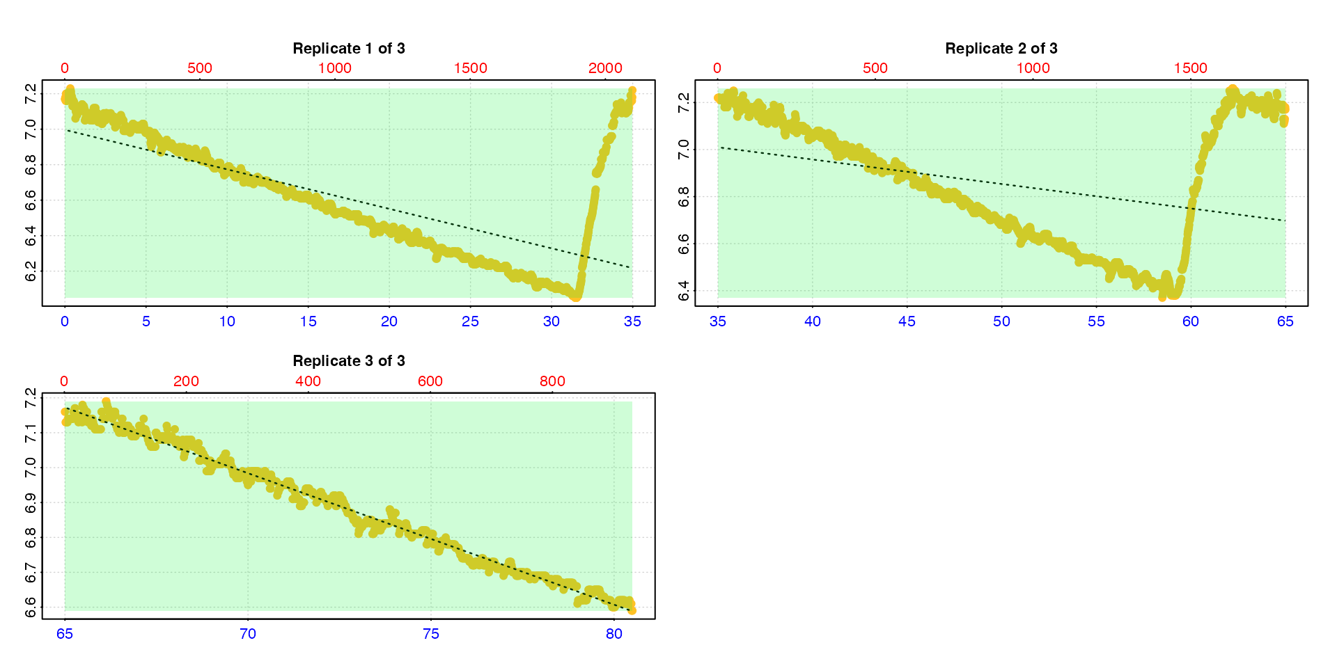

This is obviously not going to produce an appropriate rate. To exclude flush periods use the measure input. Here, using a vector of the same length as starts we can specify a different measure phase in each replicate. The default is to specify this in row widths, that is by = "row".

calc_rate.int(urchin,
              starts = c(1, 2101, 3901),
              measure = c(1800, 1200, 800))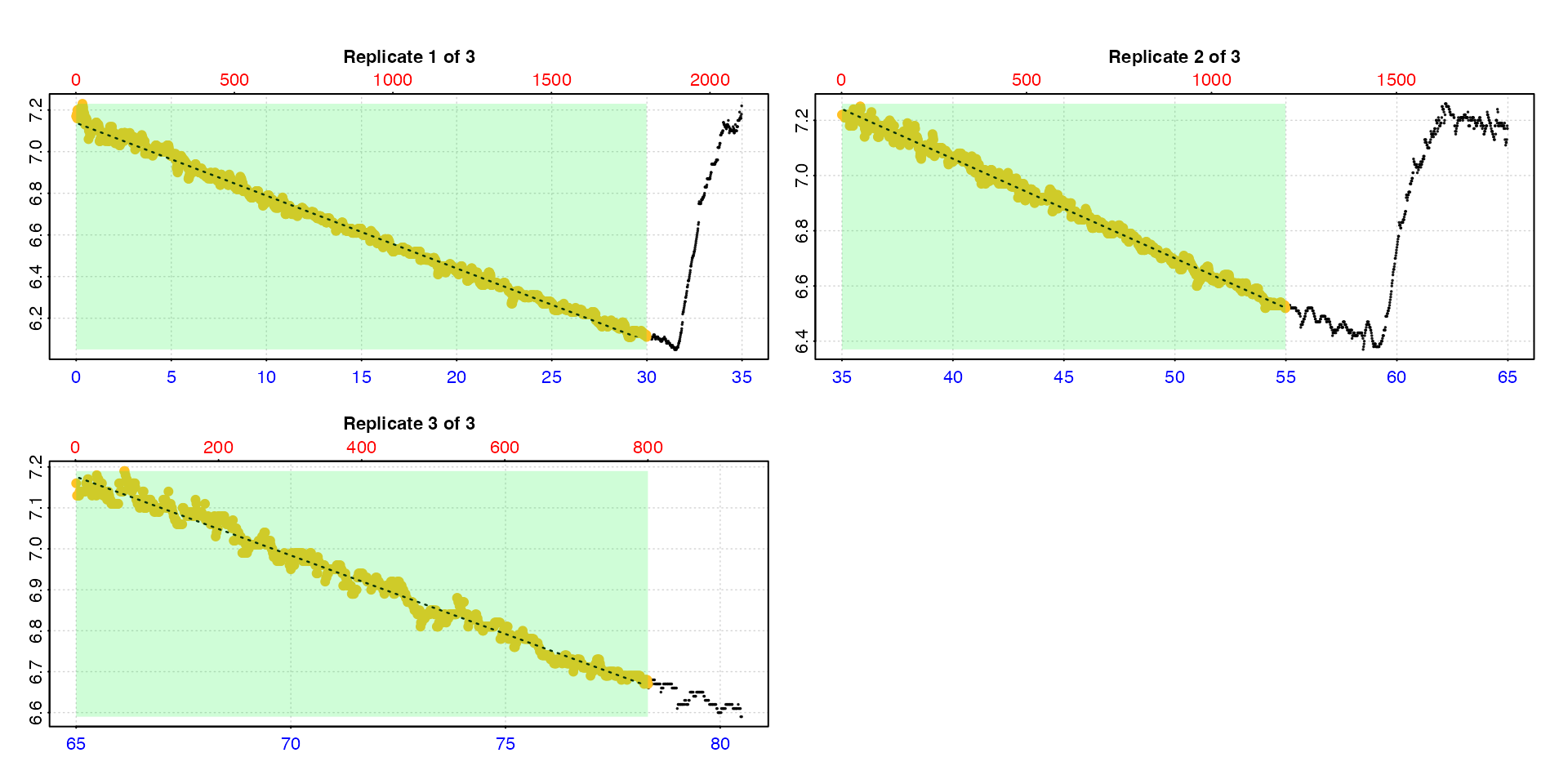

However, we usually want to use the same region within each replicate to get a rate, and also exclude the first few minutes to allow a period of settling or acclimation after the flush. We can enter the wait and measure inputs as single values to acheive this.

calc_rate.int(urchin,
              starts = c(1, 2101, 3901),
              wait = 180,
              measure = 600)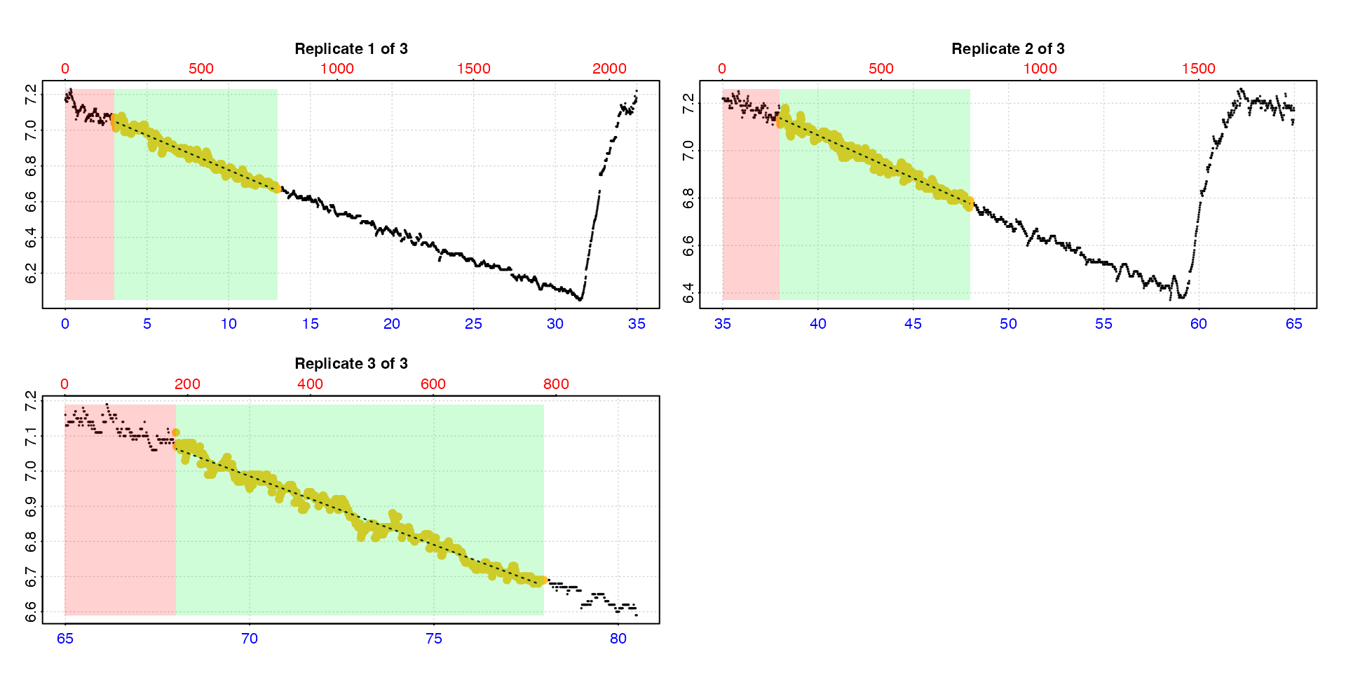

Rate from `time` range in each replicate

starts, wait, and measure can also be specified in the time units of the original data by using by = "time".

calc_rate.int(urchin,
              starts = c(0,35,64),
              wait = 3,
              measure = 10,
              by = "time")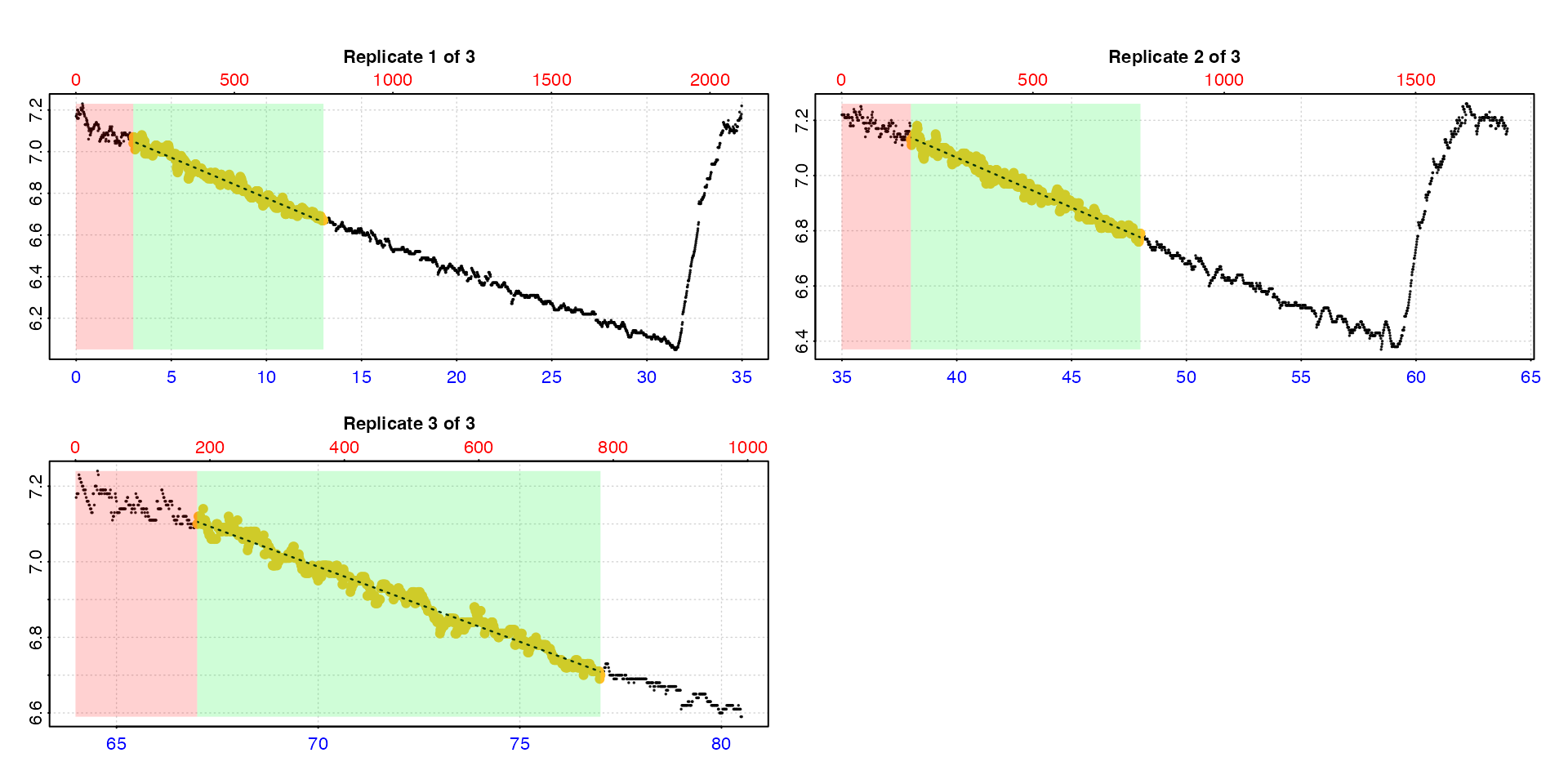

The function uses the closest matching values if the exact values do not occur in the time data.

Regularly spaced replicates

For intermittent-flow experiments where the replicates are regularly spaced you do not have to specify the start location of every single one in starts. You can instead enter a value specifying the interval between each replicate starting at the first row of the input data in either rows or time units, as specified via the by input.

Specify regular replicate structure

The zeb_intermittent.rd data is from an intermittent-flow experiment on a zebrafish. It has a regular replicate cycle of 11 minutes (660 rows) for most of its length, comprising 9 minutes of measuring and 2 minutes flush. See help("zeb_intermittent.rd") for exact locations, but essentially after a background control and a single replicate of 14 minutes this cycle is maintained until the background recording at the end.

Here we use subset_data() to extract only the regularly spaced replicates, and pipe the result to calc_rate.int. We specify the 660 row cycle using starts, exclude the first 2 minutes of each replicate using wait, and extract a rate from the following 6 minutes using measure, leaving the flush excluded.

zeb_all <- zeb_intermittent.rd |>
  
  # inspect the data
  inspect() |>
  
  # subset regular replicates from larger dataset
  subset_data(from = 5840,
              to = 75139,
              by = "row",
              quiet = TRUE) |>
  
  # calc rate in each one from row 120 to 480, plotting first 3 and last 3
  calc_rate.int(
    starts = 660,
    wait = 120,
    measure = 360, 
    by = "row",
    plot = TRUE,
    pos = c(1:3, 103:105))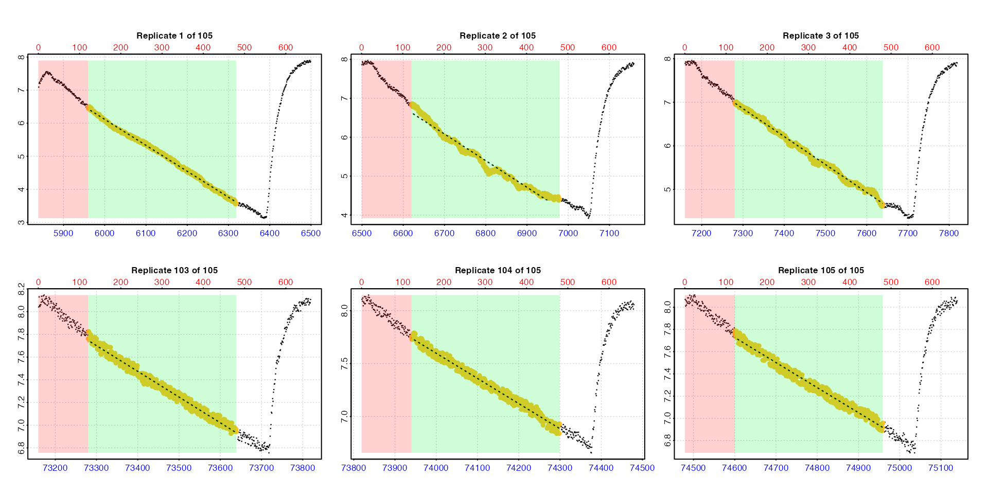

We use the pos input which is passed to plot to select the first and last three replicates for plotting to check everything looks okay. In a full analysis however we strongly recommend every replicate rate result be examined visually. Up to 20 results at a time can be plotted using the pos input. See Plot section below for further details.

View summary

Each replicate result is saved in the $summary element of the output, or we can use summary().

summary(zeb_all)
#> 
#> # summary.calc_rate.int # ---------------
#> Summary of all replicate results:
#> 
#>      rep rank intercept_b0 slope_b1   rsq   row endrow  time endtime  oxy endoxy rate.2pt     rate
#>   1:   1    1         53.2 -0.00785 0.997   121    480  5960    6319 6.45   3.57 -0.00804 -0.00785
#>   2:   2    1         51.9 -0.00684 0.975   781   1140  6620    6979 6.82   4.41 -0.00672 -0.00684
#>   3:   3    1         53.6 -0.00641 0.994  1441   1800  7280    7639 6.99   4.64 -0.00654 -0.00641
#>   4:   4    1         42.1 -0.00442 0.989  2101   2460  7940    8299 7.16   5.45 -0.00478 -0.00442
#>   5:   5    1         40.0 -0.00382 0.989  2761   3120  8600    8959 7.31   5.88 -0.00397 -0.00382
#>  ---                                                                                              
#> 101: 101    1        169.3 -0.00225 0.982 66121  66480 71960   72319 7.81   6.94 -0.00241 -0.00225
#> 102: 102    1        178.1 -0.00235 0.984 66781  67140 72620   72979 7.77   6.88 -0.00250 -0.00235
#> 103: 103    1        173.6 -0.00226 0.982 67441  67800 73280   73639 7.76   6.94 -0.00229 -0.00226
#> 104: 104    1        183.5 -0.00238 0.984 68101  68460 73940   74299 7.75   6.93 -0.00229 -0.00238
#> 105: 105    1        175.9 -0.00225 0.980 68761  69120 74600   74959 7.76   6.96 -0.00224 -0.00225
#> -----------------------------------------

The replicate number is indicated by the $rep column. The $rank column indicates ranking or ordering of rates within each individual replicate. Since calc_rate.int only returns one rate per replicate it is not relevant here, but is useful for auto_rate.int() results where multiple rates per replicate may be returned.

Plot

If plot = TRUE, a plot is produced of each replicate rate result on a grid up to a total of 20. By default this is the first 20 (i.e. pos = 1:20). Others can be selected by modifying the pos input, either in the main function call or when calling plot() on output objects.

plot(zeb_all, pos = 50:69)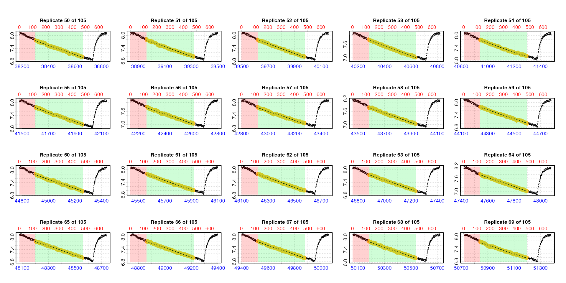

For all plots, the bottom blue time axis shows the time values of the original larger dataset, whilst the upper red row axis shows the rows of the replicate subset.

There are three ways in which these calc_rate.int results can be plotted, selected using the type input in either the main function call or when calling plot() on output objects.

`type = "rep"`

The default is type = "rep" in which each replicate is plotted individually with the rate region highlighted.

calc_rate.int(urchin,
              starts = c(0,35,64),
              wait = 5,
              measure = 15,
              by = "time")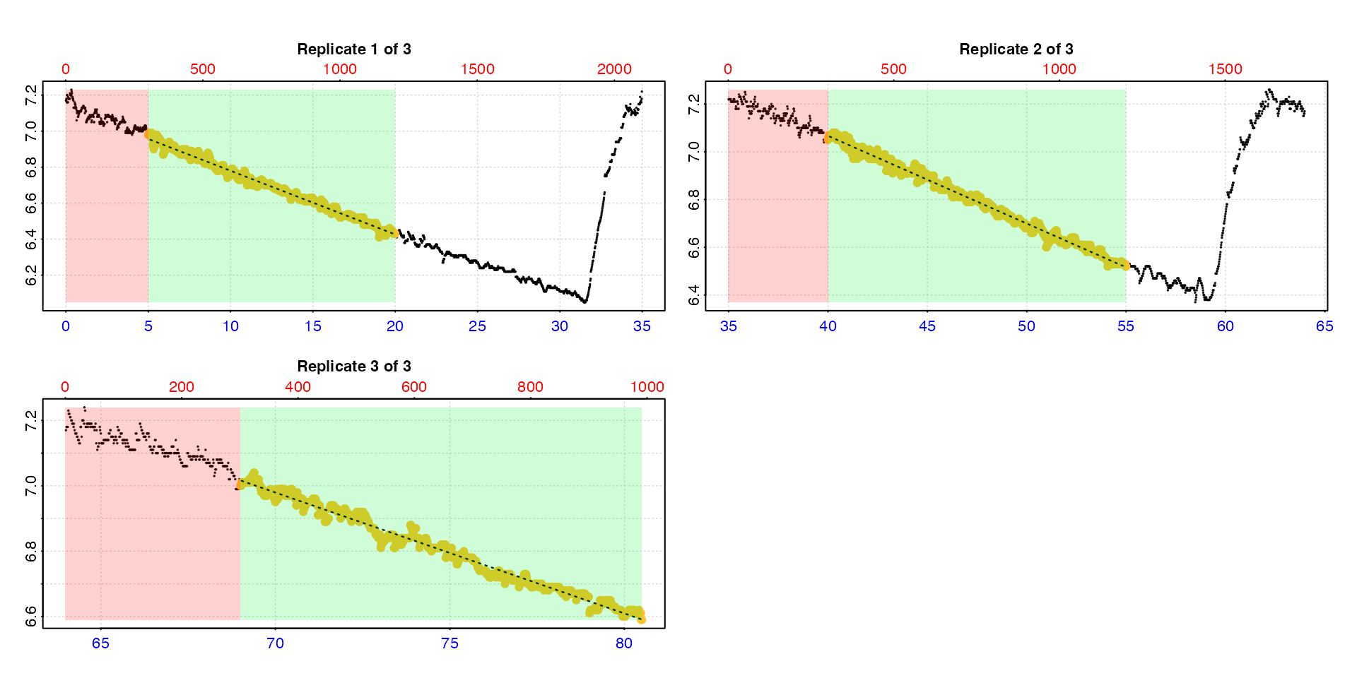

`type = "full"`

Entering type = "full" will show each replicate rate highlighted in the context of the entire dataset.

calc_rate.int(urchin,
              starts = c(0,35,64),
              wait = 5,
              measure = 15,
              by = "time",
              type = "full")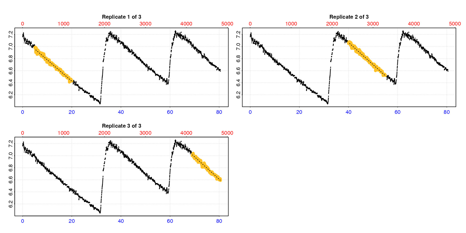

Note this may be of limited use when the dataset is large.

plot(zeb_all, type = "full", pos = 50)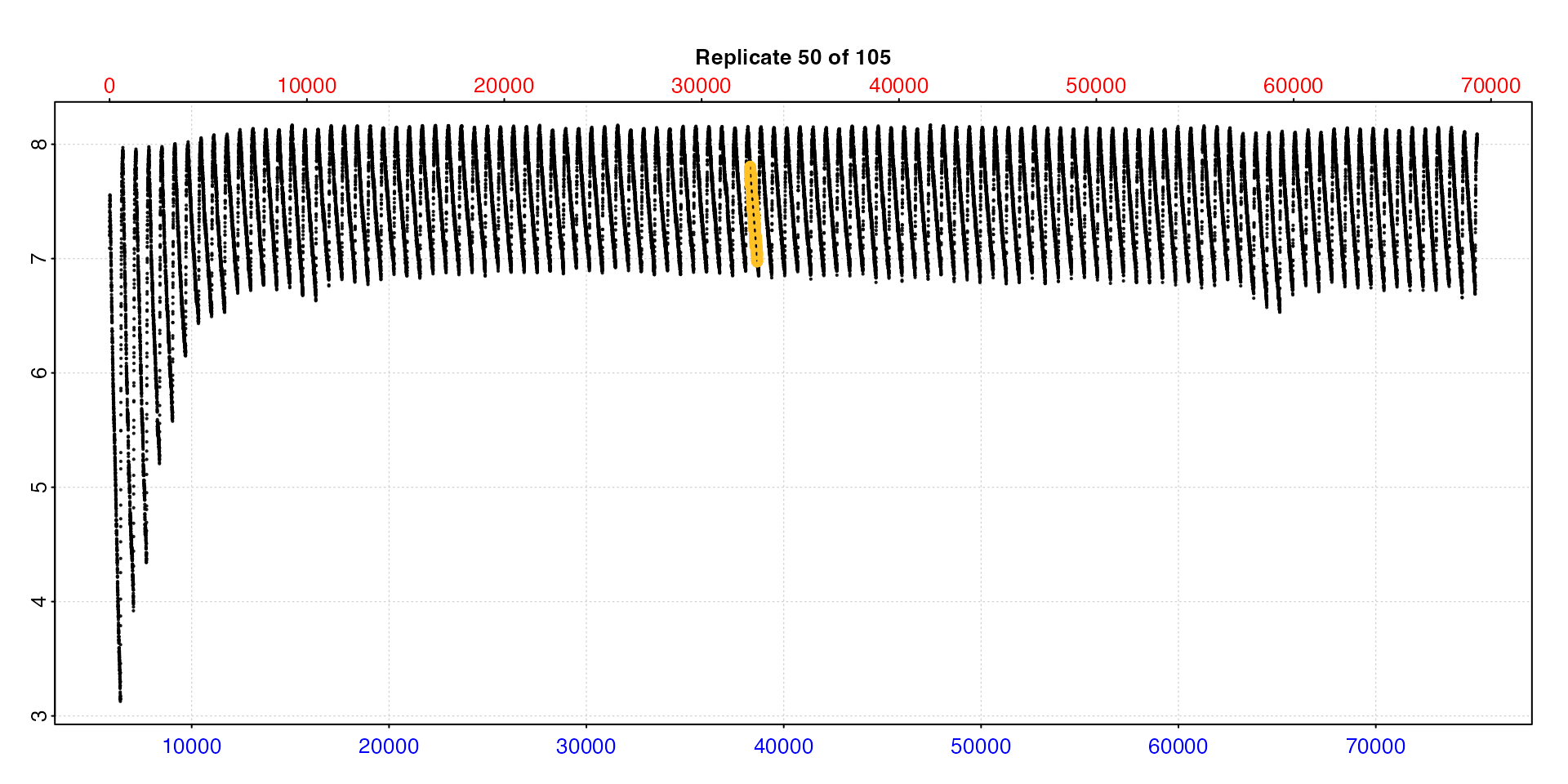

`type = "cr"`

Lastly, the calc_rate result for each individual replicate (as found in the $results element of the output) can be plotted using type = "cr" and the pos input. Note these are results from subsets of the initial data.

plot(zeb_all, type = "cr", pos = 50)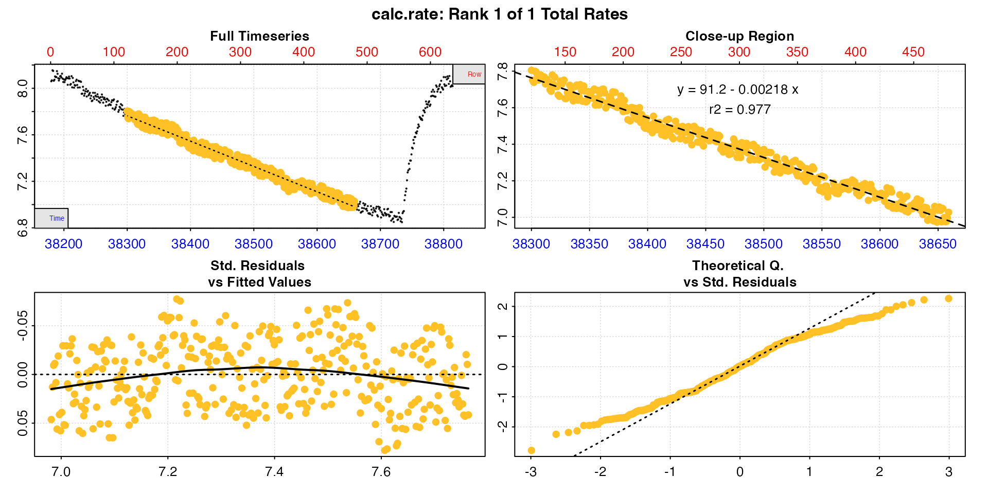

The pos input here can also be of multiple replicates but this will produce multiple individual plots that you will need to scroll through.

Additional plotting options

legend can be used to show axis labels (default is FALSE). quiet suppresses console output. Additional plotting parameters can also be passed to adjust margins, axis label rotation, etc. See here.

S3 generic methods

As well as plot, saved calc_rate.int objects work with the generic S3 methods print, summary, and mean

`print`

This simply prints a single replicate rate result to the console, by default the first one. The pos input can be used to print others.

print(zeb_all)
#> 
#> # print.calc_rate.int # -----------------
#> Replicate 1 of 105 :
#> Rate: -0.00785 
#> 
#> To see other replicate results use 'pos' input. 
#> To see full results use summary().
#> -----------------------------------------
print(zeb_all, pos = 50)
#> 
#> # print.calc_rate.int # -----------------
#> Replicate 50 of 105 :
#> Rate: -0.00218 
#> 
#> To see other replicate results use 'pos' input. 
#> To see full results use summary().
#> -----------------------------------------

`summary`

This prints the summary table to the console which contains linear model coefficients and other metadata for each replicate rate. The pos input can be used to select which replicates ($rep column) to include.

summary(zeb_all)
#> 
#> # summary.calc_rate.int # ---------------
#> Summary of all replicate results:
#> 
#>      rep rank intercept_b0 slope_b1   rsq   row endrow  time endtime  oxy endoxy rate.2pt     rate
#>   1:   1    1         53.2 -0.00785 0.997   121    480  5960    6319 6.45   3.57 -0.00804 -0.00785
#>   2:   2    1         51.9 -0.00684 0.975   781   1140  6620    6979 6.82   4.41 -0.00672 -0.00684
#>   3:   3    1         53.6 -0.00641 0.994  1441   1800  7280    7639 6.99   4.64 -0.00654 -0.00641
#>   4:   4    1         42.1 -0.00442 0.989  2101   2460  7940    8299 7.16   5.45 -0.00478 -0.00442
#>   5:   5    1         40.0 -0.00382 0.989  2761   3120  8600    8959 7.31   5.88 -0.00397 -0.00382
#>  ---                                                                                              
#> 101: 101    1        169.3 -0.00225 0.982 66121  66480 71960   72319 7.81   6.94 -0.00241 -0.00225
#> 102: 102    1        178.1 -0.00235 0.984 66781  67140 72620   72979 7.77   6.88 -0.00250 -0.00235
#> 103: 103    1        173.6 -0.00226 0.982 67441  67800 73280   73639 7.76   6.94 -0.00229 -0.00226
#> 104: 104    1        183.5 -0.00238 0.984 68101  68460 73940   74299 7.75   6.93 -0.00229 -0.00238
#> 105: 105    1        175.9 -0.00225 0.980 68761  69120 74600   74959 7.76   6.96 -0.00224 -0.00225
#> -----------------------------------------
summary(zeb_all, pos = 1:4)
#> 
#> # summary.calc_rate.int # ---------------
#> Summary of results from entered 'pos' replicate(s):
#> 
#>    rep rank intercept_b0 slope_b1   rsq  row endrow time endtime  oxy endoxy rate.2pt     rate
#> 1:   1    1         53.2 -0.00785 0.997  121    480 5960    6319 6.45   3.57 -0.00804 -0.00785
#> 2:   2    1         51.9 -0.00684 0.975  781   1140 6620    6979 6.82   4.41 -0.00672 -0.00684
#> 3:   3    1         53.6 -0.00641 0.994 1441   1800 7280    7639 6.99   4.64 -0.00654 -0.00641
#> 4:   4    1         42.1 -0.00442 0.989 2101   2460 7940    8299 7.16   5.45 -0.00478 -0.00442
#> -----------------------------------------

export = TRUE can be used to export the summary table as a data frame, or those rows selected using pos

zeb_exp <- summary(zeb_all, 
                   pos = 1:4, 
                   export = TRUE)

zeb_exp
#>    rep rank intercept_b0 slope_b1   rsq  row endrow time endtime  oxy endoxy rate.2pt     rate
#> 1:   1    1         53.2 -0.00785 0.997  121    480 5960    6319 6.45   3.57 -0.00804 -0.00785
#> 2:   2    1         51.9 -0.00684 0.975  781   1140 6620    6979 6.82   4.41 -0.00672 -0.00684
#> 3:   3    1         53.6 -0.00641 0.994 1441   1800 7280    7639 6.99   4.64 -0.00654 -0.00641
#> 4:   4    1         42.1 -0.00442 0.989 2101   2460 7940    8299 7.16   5.45 -0.00478 -0.00442

`mean`

This averages all replicate rates in the $rate column, or those selected using pos. The result can be saved as a value by using export = TRUE.

zeb_mean <- mean(zeb_all, pos = 1:4, export = TRUE)
#> 
#> # mean.calc_rate.int # ------------------
#> Mean of rate results from entered 'pos' replicates:
#> 
#> Mean of 4 replicate rates:
#> [1] -0.00638
#> -----------------------------------------
zeb_mean
#> [1] -0.00638

This could be passed as a numeric value to later functions such as convert_rate(), although it is usually better to do this kind of result filtering after conversion.

Notes and tips

Internally calc_rate.int uses calc_rate() to extract rates, which explains why each replicate result in $results is a calc_rate object. The wait and measure inputs are simply converted to the from and to inputs of calc_rate. Essentially from is equivalent to wait, and to equivalent to wait + measure. If you want to use the by = "oxygen" method of calc_rate you will have to look into looping the function. See here.
Note the default behaviour of calc_rate if values are outside the range present within each replicate is used. For example if the entered measure phase is longer than the actual replicate, the last row or time value in the replicate will be used instead. Similarly, if wait or measure inputs do not match exactly to a value within the data the closest matching value is used instead. See calc_rate() for full details.
The examples above assume flushes occur at the end of each replicate. If your data is subset or processed so that flushes are at the start instead this is easy to deal with. Simply use wait to exclude the flush at the start plus whatever subsequent wait phase you want to use before the measure phase. See example here.