
Run auto_rate on multiple replicates in intermittent-flow respirometry data
Source:R/auto_rate.int.R
auto_rate.int.Rdauto_rate.int allows you to run the auto_rate() function on multiple
replicates in intermittent-flow respirometry. A wait and measure phase
can be specified for each replicate, and the auto_rate analysis is
performed within the measure region.
Usage
auto_rate.int(
  x,
  starts = NULL,
  wait = NULL,
  measure = NULL,
  by = "row",
  method = "linear",
  width = NULL,
  n = 1,
  plot = TRUE,
  ...
)
Arguments
- x
object of class
inspectordata.frame. This is the timeseries of paired values of oxygen against time containing multiple replicates from which to calculate rates.- starts
Numeric. Row locations or times (in the units of the data in
x) of the start of each replicate. If a single value it indicates a regular interval in rows or time starting from row 1. If a vector, each entry is the start row or time of an individual replicate. Use of rows or time is controlled viaby.- wait
Numeric. A row length or time duration to be applied at the start of each replicate to exclude these data from any rate calculations. Can be a single value to apply the same wait phase to each replicate, or a vector of the same length as
startsof different wait phases for each replicate. Optional.- measure
Numeric. A row length or time duration to be applied at the end of the
waitphase (if used), and used to exclude the flush period. This is the region within which theauto_rateanalysis is conducted for each replicate. Can be a single value to apply the same measure phase to each replicate, or a vector of the same length asstartsof different measure phases for each replicate. Default isNULLin which case the entire replicate is used (which is rarely what is wanted).- by
String.
"row"or"time". Controls howstarts,waitandmeasureare applied. It also controls how thewidthis applied in theauto_rateanalysis - seehelp("auto_rate"). Default is"row".- method
string. The
auto_ratemethodto use. Default is"linear". Others include"lowest"and"highest". Seehelp("auto_rate")for descriptions and other methods.- width
numeric. The
widthto use in theauto_rateanalysis. Mandatory and should be entered in the correct units of thebyinput. Seehelp("auto_rate")and vignettes on website for how width affects analyses.- n
integer. How many
auto_rateresults to return for each replicate. Default is1.- plot
logical. Default is
TRUE. Plots the results. See 'Plotting' section for details.- ...
Allows additional plotting controls to be passed, such as
type,pos,legend, andquiet.
Value
Output is a list object of class auto_rate.int containing a
auto_rate object for each replicate in $results. The output also
contains a $summary table which includes the full rate regression results
from each replicate with replicate number indicated by the $rep column.
Output also contains a $rate element which contains the rate values from
each replicate in order. The function call, inputs, and other metadata are
also included. Note, that if you have many replicates this object can be
rather large (several MB).
Details
auto_rate.int uses the starts input to subset each replicate. The wait
and measure inputs control which parts of each replicate data are excluded
and included from the rate calculation. It runs auto_rate on the measure
phase in each replicate saving the top n ranked results and extracting the
rate and other data to a summary table.
The x input should be aninspect object. Alternatively, it can be a
two-column data frame containing paired values of time and oxygen from an
intermittent-flow experiment in columns 1 and 2 respectively (though we
always recommend processing such data in inspect() first). If a multiple
column dataset is entered as x the first two columns are selected by
default. If these are not the intended data use inspect to select the
correct time and oxygen columns.
auto_rate inputs
You should be familiar with how auto_rate works before using this function.
See help("auto_rate") and vignettes on the website for full details.
The auto_rate inputs can be changed by entering different method and
width inputs. The by input controls how the width is applied. Note if
using a proportional width input (i.e. between 0 and 1 representing a
proportion of the data length) this applies to the length of the measure
phase of each particular replicate.
The n input controls how many auto_rate results from each replicate to
return in the output. By default this is only the top ranked result for the
particular method, i.e. n = 1. This can be changed to return more,
however consider carefully if this is necessary as the output will
necessarily contain many more rate results which may make it difficult to
explore and select results (although see select_rate()).
Specifying replicate structure
The starts input specifies the locations of the start of each replicate in
the data in x. This can be in one of two ways:
A single numeric value specifying the number of rows in each replicate starting from the data in the first row. This option should only be used when replicates cycle at regular intervals. This can be a regular row or time interval, as specified via the
byinput. If the first replicate does not start at row 1, the data should be subset so that it does (seesubset_data()) and example here. For example,starts = 600, by = "row"means the first replicate starts at row 1 and ends at row 600, the second starts at row 601 ends at 1200, and so on.A numeric vector of row locations or times, as specified via the
byinput, of the start of each individual replicate. The first replicate does not have to start at the first row of the data, and all data after the last entry is assumed to be part of the final replicate. RegularRsyntax such asseq(),1:10, etc. is also accepted, so can be used to specify both regular and irregular replicate spacing.
For both methods it is assumed each replicate ends at the row preceding the
start of the next replicate, or in the case of the last replicate the final
row of the dataset. Also for both methods, by = "time" inputs do not need
to be exact; the closest matching values in the time data are used.
Results are presented in the summary table with rep and rank columns to
distinguish those from different replicates and their ranking within
replicates (if multiple results per replicate have been returned by
increasing the n input).
Specifying rate region
The wait and measure inputs are used to specify the region from which to
extract a rate and exclude flush periods. They can be entered as row
intervals or time values in the units of the input data. The wait phase
controls the amount of data at the start of each replicate to be ignored,
that is excluded from any rate calculations. The measure phase determines
the region after this from which a rate is calculated. Unlike
calc_rate.int(), auto_rate.int will not necessarily use all of the data
in the measure phase, but will run the auto_rate analysis within it
using the method, width and by inputs. This may result in rates of
various widths depending on the inputs. See auto_rate() for defaults and
full details of how selection inputs are applied.
There is no flush phase input since this is assumed to be from the end of
the measure phase to the end of the replicate.
Both wait and measure can be entered in one of two ways:
Single numeric values specifying a row width or a time period, as specified via the
byinput. Use this if you want to use the samewaitandmeasurephases in every replicate.If
startsis a vector of locations of the start of each replicate, these inputs can also be vectors of equal length of row lengths or time periods as specified via thebyinput. This is only useful if you want to use differentwaitand/ormeasurephases in different replicates.
If wait = NULL no wait phase is applied. If measure = NULL the data used
for analysis is from the start of the replicate or end of the wait phase to
the last row of the replicate. This will typically include the flush period,
so is rarely what you would want.
Example
See examples below for actual code, but here is a simple example. An
experiment comprises replicates which cycle at ten minute intervals with data
recorded every second. Therefore each replicate will be 600 rows long.
Flushes of the respirometer take 3 minutes at the end of each replicate. We
want to exclude the first 2 minutes (120 rows) of data in each, and run an
auto_rate analysis to get an oxygen uptake rate within the following five
minute period (300 rows), leaving the three minutes of flushing (180 rows)
excluded. The inputs for this would be:
starts = 600, wait = 120, measure = 300, by = "row"
Plot
If plot = TRUE (the default), the result for each rate is plotted on a grid
up to a maximum of 20. There are three ways of plotting the results, which
can be selected using the type input:
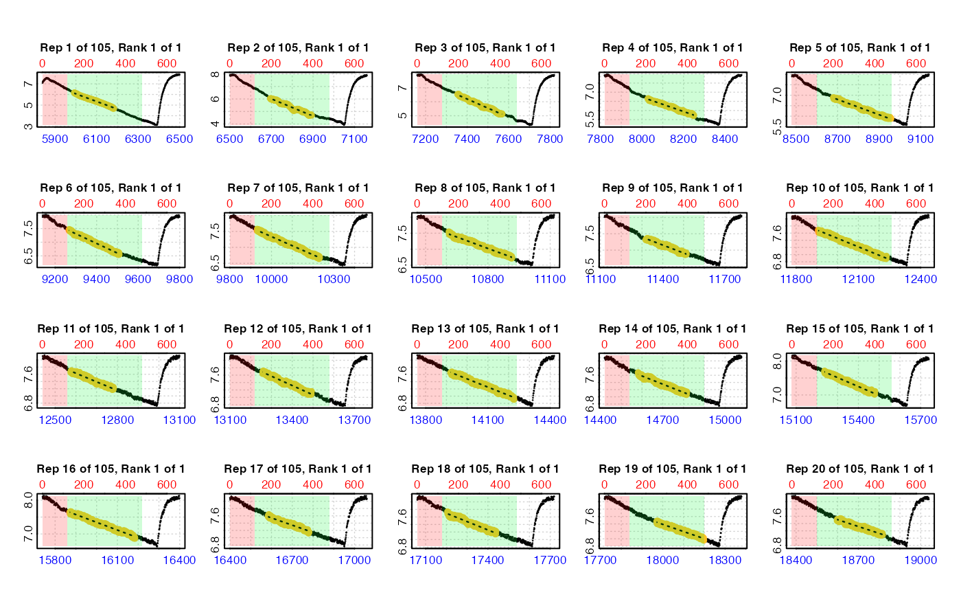
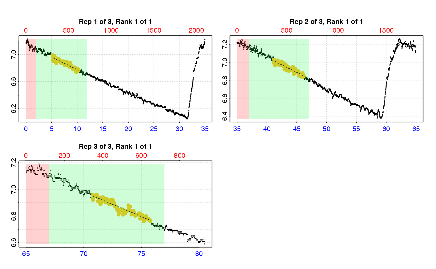
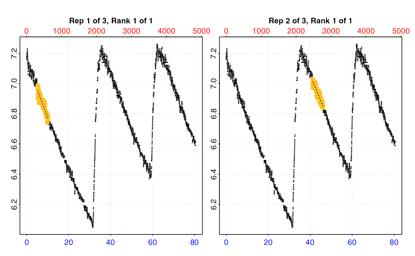
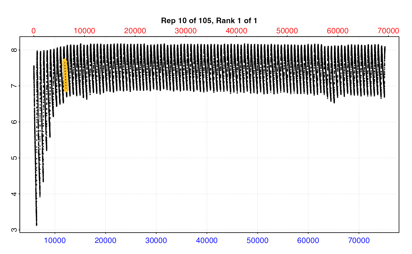
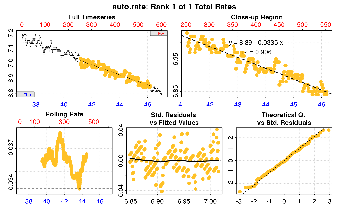
type = "rep": The default. Each individual replicate is plotted with the rate region highlighted in yellow. Thewaitandmeasurephases are also highlighted as shaded red and green regions respectively. These are also labelled iflegend = TRUE.type = "full": Each replicate rate is highlighted in the context of the whole dataset. May be quite difficult to interpret if dataset is large.type = "ar": Plots individual replicate results asauto_rateobjects. Note, these will only show themeasurephase of the data.
For all plot types pos can be used to select which rate(s) to plot (default
is 1:20), where pos indicates rows of the $summary table (and hence which
$rep and $rank). This can be passed either in the main function call or
when calling plot() on output objects. Note for all plot types if n has
been changed to return more than one rate per replicate these will also be
plotted.
S3 Generic Functions
Saved output objects can be used in the generic S3 functions plot(),
print(), summary(), and mean(). For all of these pos selects rows of
the $summary table.
plot(): plots the result. See Plot section above.print(): prints the result of a single rate, by default the first. Others can be printed by passing theposinput. e.g.print(x, pos = 2)summary(): prints summary table of all results and metadata, or the rows specified by theposinput. e.g.summary(x, pos = 1:5). The$repcolumn indicates the replicate number, and$rankcolumn the ranking of each rate within each replicate (only used if a differentnhas been passed, otherwise they are all1). The summary table (orposrows) can be exported as a separate data frame by passingexport = TRUE.mean(): calculates the mean of the rates from every row or those specified by theposinput. e.g.mean(x, pos = 1:5)Note if a differentnhas been passed this may include multiple rates from each replicate. The mean can be exported as a numeric value by passingexport = TRUE.
More
For additional help, documentation, vignettes, and more visit the respR
website at https://januarharianto.github.io/respR/
Examples
# \donttest{
# Irregular replicate structure ------------------------------------------
# Prepare the data to use in examples
# Note in this dataset each replicate is a different length!
data <- intermittent.rd
# Convert time to minutes (to show different options below)
data[[1]] <- round(data[[1]]/60, 2)
# Inspect
urch_insp <- inspect(data)
#> inspect: Applying column default of 'time = 1'
#> inspect: Applying column default of 'oxygen = 2'
#> Warning: inspect: Time values are not evenly-spaced (numerically).
#> inspect: Data issues detected. For more information use print().
#>
#> # print.inspect # -----------------------
#> Time O2
#> numeric pass pass
#> Inf/-Inf pass pass
#> NA/NaN pass pass
#> sequential pass -
#> duplicated pass -
#> evenly-spaced WARN -
#>
#> Uneven Time data locations (first 20 shown) in column: Time
#> [1] 1 2 3 4 5 6 7 8 9 10 11 12 13 14 15 16 17 18 19 20
#> Minimum and Maximum intervals in uneven Time data:
#> [1] 0.01 0.02
#> -----------------------------------------
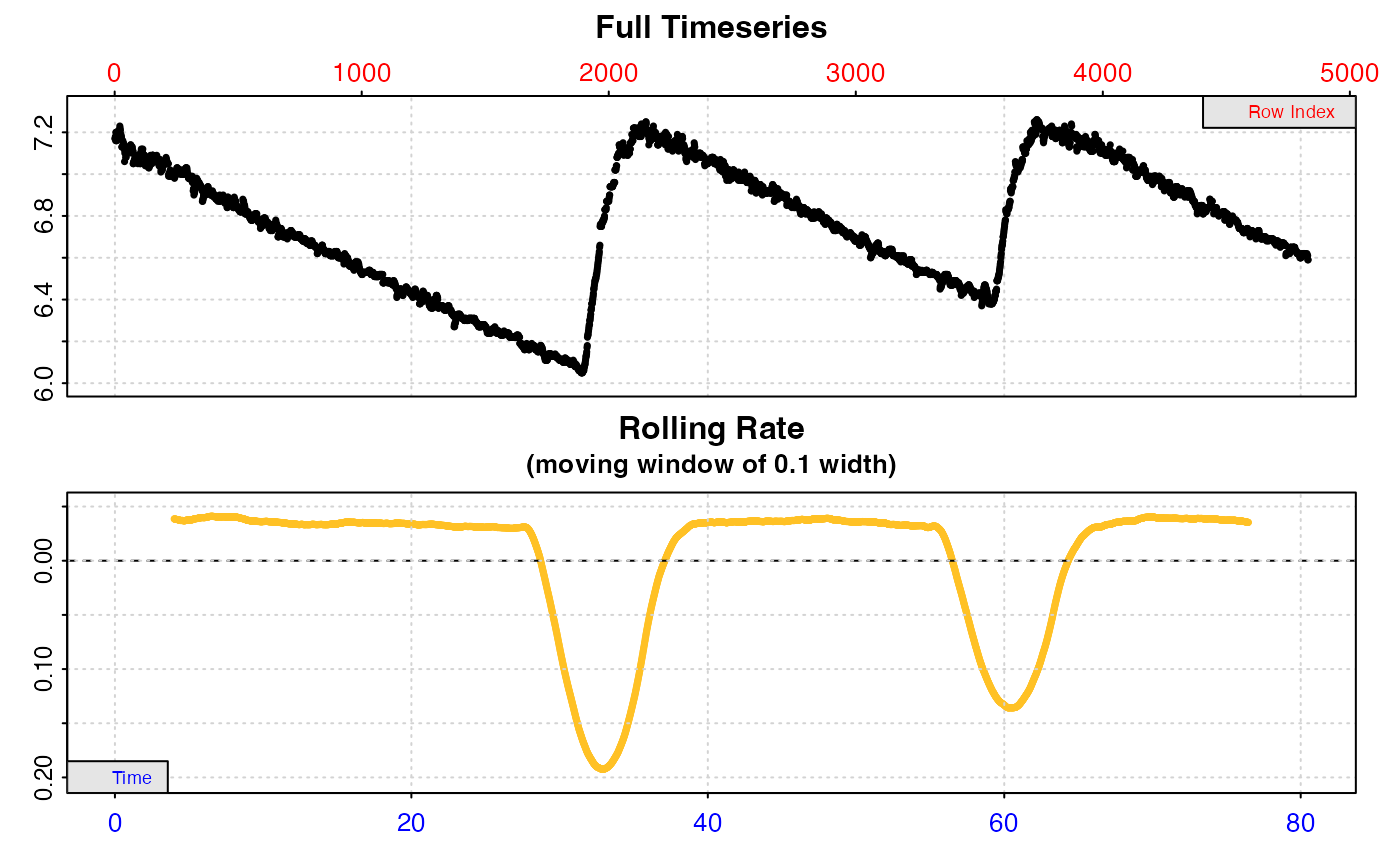 # Calculate the most linear rate within each replicate
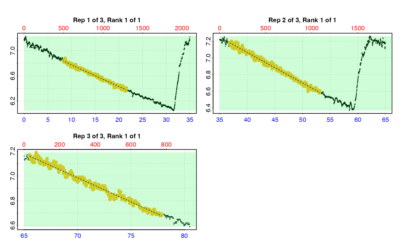
auto_rate.int(urch_insp,
starts = c(1, 2101, 3901),
by = "row",
method = "linear",
width = 400) %>%
summary()
#> auto_rate.int: The `measure` input is NULL. Calculating rate to the end of the replicate.
#>
#> # plot.auto_rate.int # ------------------
#> plot.auto_rate.int: Plotting all rates ...
 #> -----------------------------------------
#>
#> # summary.auto_rate.int # ---------------
#> Summary of all rate results:
#>
#> rep rank intercept_b0 slope_b1 rsq density row endrow time endtime oxy endoxy rate
#> 1: 1 1 7.118754 -0.03441525 0.988 125.9405 495 1291 8.23 21.50 6.84 6.40 -0.03441525
#> 2: 2 1 8.528343 -0.03659034 0.991 191.1540 2205 3188 36.73 53.12 7.17 6.60 -0.03659034
#> 3: 3 1 9.718837 -0.03904824 0.984 391.0745 3930 4673 65.48 77.87 7.18 6.69 -0.03904824
#> -----------------------------------------
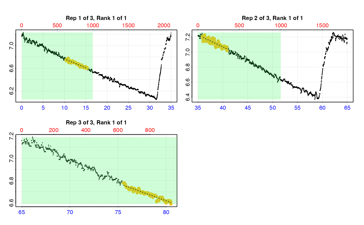
# Calculate the lowest rate within each replicate across
# 5 minutes (300 rows). For this we need to specify a 'measure' phase
# so that the flush is excluded.
auto_rate.int(urch_insp,
starts = c(1, 2101, 3901),
measure = 1000,
by = "row",
method = "lowest",
width = 300) %>%
summary()
#>
#> # plot.auto_rate.int # ------------------
#> plot.auto_rate.int: Plotting all rates ...
#> -----------------------------------------
#>
#> # summary.auto_rate.int # ---------------
#> Summary of all rate results:
#>
#> rep rank intercept_b0 slope_b1 rsq density row endrow time endtime oxy endoxy rate
#> 1: 1 1 7.118754 -0.03441525 0.988 125.9405 495 1291 8.23 21.50 6.84 6.40 -0.03441525
#> 2: 2 1 8.528343 -0.03659034 0.991 191.1540 2205 3188 36.73 53.12 7.17 6.60 -0.03659034
#> 3: 3 1 9.718837 -0.03904824 0.984 391.0745 3930 4673 65.48 77.87 7.18 6.69 -0.03904824
#> -----------------------------------------
# Calculate the lowest rate within each replicate across
# 5 minutes (300 rows). For this we need to specify a 'measure' phase
# so that the flush is excluded.
auto_rate.int(urch_insp,
starts = c(1, 2101, 3901),
measure = 1000,
by = "row",
method = "lowest",
width = 300) %>%
summary()
#>
#> # plot.auto_rate.int # ------------------
#> plot.auto_rate.int: Plotting all rates ...
 #> -----------------------------------------
#>
#> # summary.auto_rate.int # ---------------
#> Summary of all rate results:
#>
#> rep rank intercept_b0 slope_b1 rsq density row endrow time endtime oxy endoxy rate
#> 1: 1 1 7.073573 -0.03091433 0.9324591 NA 623 922 10.37 15.35 6.75 6.60 -0.03091433
#> 2: 2 1 8.332909 -0.03159440 0.8589605 NA 2153 2452 35.87 40.85 7.21 7.07 -0.03159440
#> 3: 3 1 9.145790 -0.03158795 0.9389333 NA 4532 4831 75.52 80.50 6.78 6.59 -0.03158795
#> -----------------------------------------
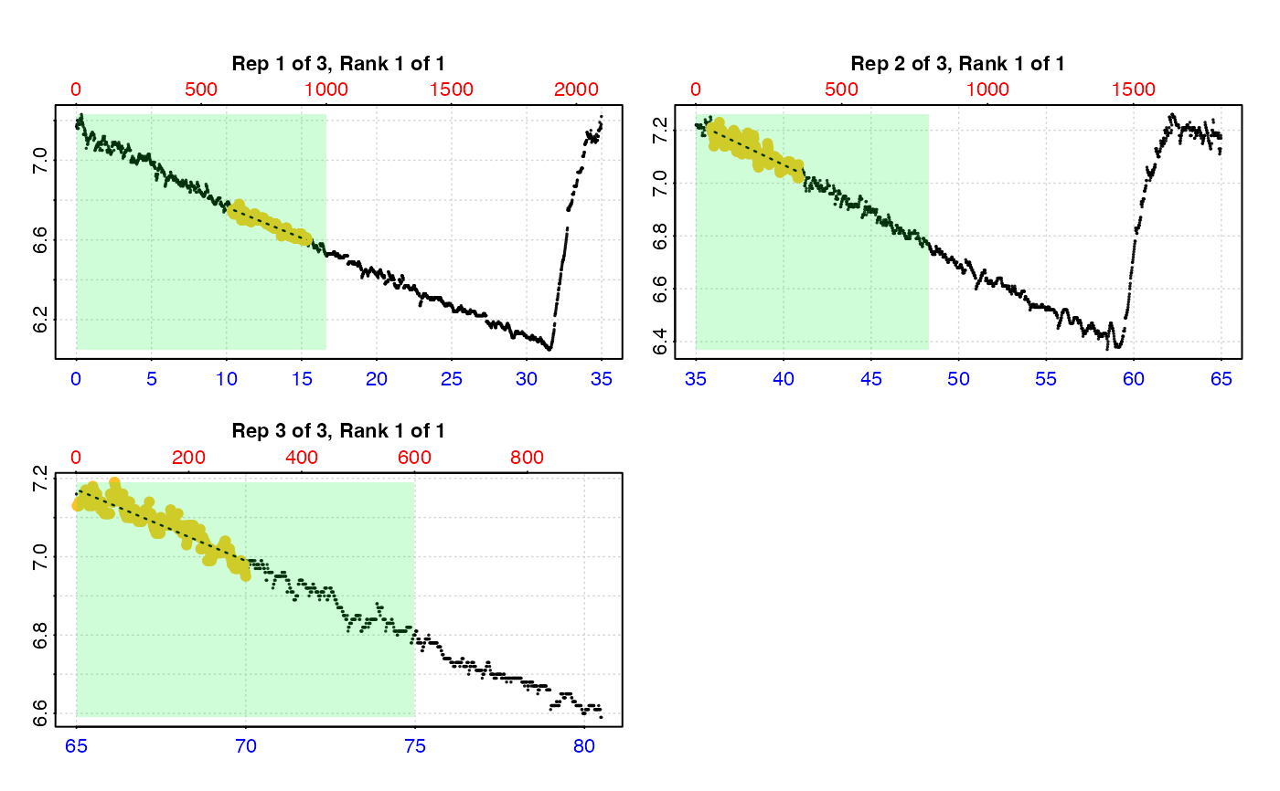
# You can even specify different 'measure' phases in each rep
auto_rate.int(urch_insp,
starts = c(1, 2101, 3901),
measure = c(1000, 800, 600),
by = "row",
method = "lowest",
width = 300) %>%
summary()
#>
#> # plot.auto_rate.int # ------------------
#> plot.auto_rate.int: Plotting all rates ...
#> -----------------------------------------
#>
#> # summary.auto_rate.int # ---------------
#> Summary of all rate results:
#>
#> rep rank intercept_b0 slope_b1 rsq density row endrow time endtime oxy endoxy rate
#> 1: 1 1 7.073573 -0.03091433 0.9324591 NA 623 922 10.37 15.35 6.75 6.60 -0.03091433
#> 2: 2 1 8.332909 -0.03159440 0.8589605 NA 2153 2452 35.87 40.85 7.21 7.07 -0.03159440
#> 3: 3 1 9.145790 -0.03158795 0.9389333 NA 4532 4831 75.52 80.50 6.78 6.59 -0.03158795
#> -----------------------------------------
# You can even specify different 'measure' phases in each rep
auto_rate.int(urch_insp,
starts = c(1, 2101, 3901),
measure = c(1000, 800, 600),
by = "row",
method = "lowest",
width = 300) %>%
summary()
#>
#> # plot.auto_rate.int # ------------------
#> plot.auto_rate.int: Plotting all rates ...
 #> -----------------------------------------
#>
#> # summary.auto_rate.int # ---------------
#> Summary of all rate results:
#>
#> rep rank intercept_b0 slope_b1 rsq density row endrow time endtime oxy endoxy rate
#> 1: 1 1 7.073573 -0.03091433 0.9324591 NA 623 922 10.37 15.35 6.75 6.60 -0.03091433
#> 2: 2 1 8.332909 -0.03159440 0.8589605 NA 2153 2452 35.87 40.85 7.21 7.07 -0.03159440
#> 3: 3 1 9.524136 -0.03620204 0.8662114 NA 3901 4200 65.00 69.98 7.16 6.96 -0.03620204
#> -----------------------------------------
# We usually don't want to use the start of a replicate just after the flush,
# so we can specify a 'wait' phase. We can also specify 'starts', 'wait',
# 'measure', and 'width' in units of time instead of rows.
#
# By time
# (this time we save the result)
urch_res <- auto_rate.int(urch_insp,
starts = c(0, 35, 65), # start locations in minutes
wait = 2, # wait for 2 mins
measure = 10, # measure phase of 10 mins
by = "time", # apply inputs by time values
method = "lowest", # get the 'lowest' rate...
width = 5) %>% # ... of 5 minutes width
summary()
#>
#> # plot.auto_rate.int # ------------------
#> plot.auto_rate.int: Plotting all rates ...
#> -----------------------------------------
#>
#> # summary.auto_rate.int # ---------------
#> Summary of all rate results:
#>
#> rep rank intercept_b0 slope_b1 rsq density row endrow time endtime oxy endoxy rate
#> 1: 1 1 7.073573 -0.03091433 0.9324591 NA 623 922 10.37 15.35 6.75 6.60 -0.03091433
#> 2: 2 1 8.332909 -0.03159440 0.8589605 NA 2153 2452 35.87 40.85 7.21 7.07 -0.03159440
#> 3: 3 1 9.524136 -0.03620204 0.8662114 NA 3901 4200 65.00 69.98 7.16 6.96 -0.03620204
#> -----------------------------------------
# We usually don't want to use the start of a replicate just after the flush,
# so we can specify a 'wait' phase. We can also specify 'starts', 'wait',
# 'measure', and 'width' in units of time instead of rows.
#
# By time
# (this time we save the result)
urch_res <- auto_rate.int(urch_insp,
starts = c(0, 35, 65), # start locations in minutes
wait = 2, # wait for 2 mins
measure = 10, # measure phase of 10 mins
by = "time", # apply inputs by time values
method = "lowest", # get the 'lowest' rate...
width = 5) %>% # ... of 5 minutes width
summary()
#>
#> # plot.auto_rate.int # ------------------
#> plot.auto_rate.int: Plotting all rates ...
 #> -----------------------------------------
#>
#> # summary.auto_rate.int # ---------------
#> Summary of all rate results:
#>
#> rep rank intercept_b0 slope_b1 rsq density row endrow time endtime oxy endoxy rate
#> 1: 1 1 7.149795 -0.03742759 0.9083621 NA 314 614 5.22 10.22 6.99 6.76 -0.03742759
#> 2: 2 1 8.393968 -0.03347137 0.9061354 NA 2472 2772 41.18 46.18 7.03 6.84 -0.03347137
#> 3: 3 1 9.548892 -0.03671394 0.8995640 NA 4248 4548 70.78 75.78 6.96 6.76 -0.03671394
#> -----------------------------------------
# Regular replicate structure --------------------------------------------
# If replicates cycle at regular intervals, 'starts' can be used to specify
# the spacing in rows or time, starting at row 1. Therefore data must be
# subset first so that the first replicate starts at row 1.
#
# Subset and inspect data
zeb_insp <- zeb_intermittent.rd %>%
subset_data(from = 5840,
to = 75139,
by = "row",
quiet = TRUE) %>%
inspect()
#> inspect: Applying column default of 'time = 1'
#> inspect: Applying column default of 'oxygen = 2'
#> inspect: No issues detected while inspecting data frame.
#>
#> # print.inspect # -----------------------
#> Time Oxygen
#> numeric pass pass
#> Inf/-Inf pass pass
#> NA/NaN pass pass
#> sequential pass -
#> duplicated pass -
#> evenly-spaced pass -
#>
#> -----------------------------------------
#> -----------------------------------------
#>
#> # summary.auto_rate.int # ---------------
#> Summary of all rate results:
#>
#> rep rank intercept_b0 slope_b1 rsq density row endrow time endtime oxy endoxy rate
#> 1: 1 1 7.149795 -0.03742759 0.9083621 NA 314 614 5.22 10.22 6.99 6.76 -0.03742759
#> 2: 2 1 8.393968 -0.03347137 0.9061354 NA 2472 2772 41.18 46.18 7.03 6.84 -0.03347137
#> 3: 3 1 9.548892 -0.03671394 0.8995640 NA 4248 4548 70.78 75.78 6.96 6.76 -0.03671394
#> -----------------------------------------
# Regular replicate structure --------------------------------------------
# If replicates cycle at regular intervals, 'starts' can be used to specify
# the spacing in rows or time, starting at row 1. Therefore data must be
# subset first so that the first replicate starts at row 1.
#
# Subset and inspect data
zeb_insp <- zeb_intermittent.rd %>%
subset_data(from = 5840,
to = 75139,
by = "row",
quiet = TRUE) %>%
inspect()
#> inspect: Applying column default of 'time = 1'
#> inspect: Applying column default of 'oxygen = 2'
#> inspect: No issues detected while inspecting data frame.
#>
#> # print.inspect # -----------------------
#> Time Oxygen
#> numeric pass pass
#> Inf/-Inf pass pass
#> NA/NaN pass pass
#> sequential pass -
#> duplicated pass -
#> evenly-spaced pass -
#>
#> -----------------------------------------
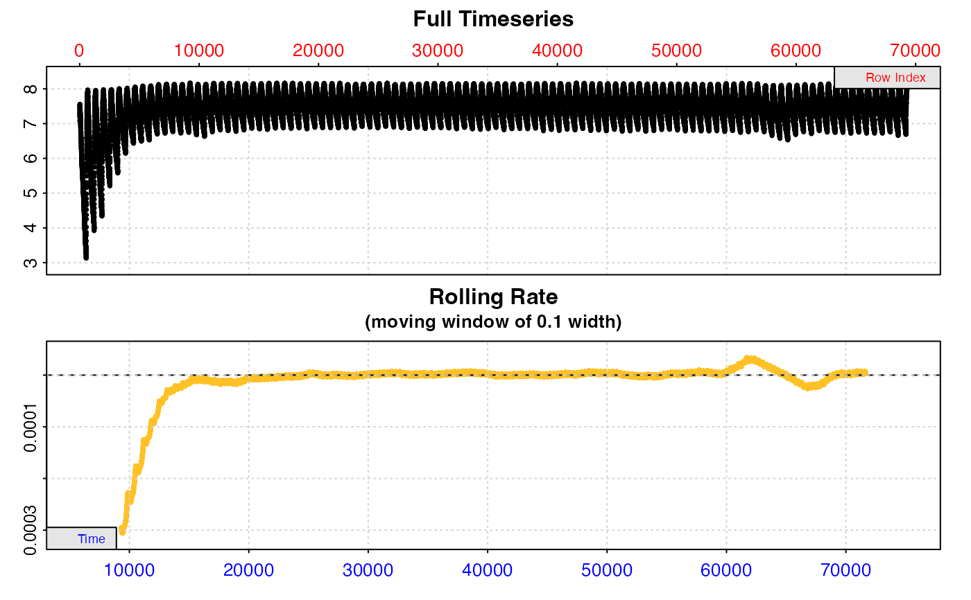 # Calculate the most linear rate from the same 6-minute region in every
# replicate. Replicates cycle at every 660 rows.
zeb_res <- auto_rate.int(zeb_insp,
starts = 660,
wait = 120, # exclude first 2 mins
measure = 360, # measure period of 6 mins after 'wait'
method = "linear",
width = 200, # starting value for linear analysis
plot = TRUE) %>%
summary()
#>
#> # plot.auto_rate.int # ------------------
#> plot.auto_rate.int: Plotting all rates ...
#> plot.auto_rate.int: Plotting first 20 selected rates only. To plot others modify 'pos' input.
 #> -----------------------------------------
#>
#> # summary.auto_rate.int # ---------------
#> Summary of all rate results:
#>
#> rep rank intercept_b0 slope_b1 rsq density row endrow time endtime oxy endoxy rate
#> 1: 1 1 49.10349 -0.007173932 0.992 2437.7265 152 343 5991 6182 6.120187 4.708402 -0.007173932
#> 2: 2 1 52.18267 -0.006891717 0.975 501.9259 854 1053 6693 6892 6.059462 4.734815 -0.006891717
#> 3: 3 1 54.30275 -0.006500972 0.987 2050.8712 1514 1729 7353 7568 6.555045 5.152687 -0.006500972
#> 4: 4 1 38.16257 -0.003929078 0.984 2222.1743 2188 2410 8027 8249 6.695938 5.704677 -0.003929078
#> 5: 5 1 38.56197 -0.003651164 0.985 8156.8732 2839 3117 8678 8956 6.872735 5.888393 -0.003651164
#> ---
#> 101: 101 1 160.84586 -0.002127990 0.965 12759.1736 66205 66460 72044 72299 7.534681 6.991055 -0.002127990
#> 102: 102 1 171.92247 -0.002260980 0.969 6226.0115 66815 67077 72654 72916 7.646181 7.036237 -0.002260980
#> 103: 103 1 171.87181 -0.002239854 0.964 17004.6247 67506 67745 73345 73584 7.634133 7.062284 -0.002239854
#> 104: 104 1 178.38106 -0.002307999 0.978 6085.5398 68136 68432 73975 74271 7.672256 6.901699 -0.002307999
#> 105: 105 1 164.49953 -0.002102029 0.954 4987.1566 68887 69120 74726 74959 7.445819 6.957930 -0.002102029
#> -----------------------------------------
# S3 functions ------------------------------------------------------------
# Outputs can be used in print(), summary(), and mean().
# 'pos' can be used to select replicate ranges
summary(zeb_res)
#>
#> # summary.auto_rate.int # ---------------
#> Summary of all rate results:
#>
#> rep rank intercept_b0 slope_b1 rsq density row endrow time endtime oxy endoxy rate
#> 1: 1 1 49.10349 -0.007173932 0.992 2437.7265 152 343 5991 6182 6.120187 4.708402 -0.007173932
#> 2: 2 1 52.18267 -0.006891717 0.975 501.9259 854 1053 6693 6892 6.059462 4.734815 -0.006891717
#> 3: 3 1 54.30275 -0.006500972 0.987 2050.8712 1514 1729 7353 7568 6.555045 5.152687 -0.006500972
#> 4: 4 1 38.16257 -0.003929078 0.984 2222.1743 2188 2410 8027 8249 6.695938 5.704677 -0.003929078
#> 5: 5 1 38.56197 -0.003651164 0.985 8156.8732 2839 3117 8678 8956 6.872735 5.888393 -0.003651164
#> ---
#> 101: 101 1 160.84586 -0.002127990 0.965 12759.1736 66205 66460 72044 72299 7.534681 6.991055 -0.002127990
#> 102: 102 1 171.92247 -0.002260980 0.969 6226.0115 66815 67077 72654 72916 7.646181 7.036237 -0.002260980
#> 103: 103 1 171.87181 -0.002239854 0.964 17004.6247 67506 67745 73345 73584 7.634133 7.062284 -0.002239854
#> 104: 104 1 178.38106 -0.002307999 0.978 6085.5398 68136 68432 73975 74271 7.672256 6.901699 -0.002307999
#> 105: 105 1 164.49953 -0.002102029 0.954 4987.1566 68887 69120 74726 74959 7.445819 6.957930 -0.002102029
#> -----------------------------------------
mean(zeb_res, pos = 1:5)
#>
#> # mean.auto_rate.int # ------------------
#> Mean of rate results from entered 'pos' rows:
#>
#> Mean of 5 rates:
#> [1] -0.005629373
#> -----------------------------------------
# There are three ways by which the results can be plotted.
# 'pos' can be used to select replicates to be plotted.
#
# type = "rep" - the default. Each replicate plotted on a grid with rate
# region highlighted (up to a maximum of 20).
plot(urch_res)
#>
#> # plot.auto_rate.int # ------------------
#> plot.auto_rate.int: Plotting all rates ...
#> -----------------------------------------
#>
#> # summary.auto_rate.int # ---------------
#> Summary of all rate results:
#>
#> rep rank intercept_b0 slope_b1 rsq density row endrow time endtime oxy endoxy rate
#> 1: 1 1 49.10349 -0.007173932 0.992 2437.7265 152 343 5991 6182 6.120187 4.708402 -0.007173932
#> 2: 2 1 52.18267 -0.006891717 0.975 501.9259 854 1053 6693 6892 6.059462 4.734815 -0.006891717
#> 3: 3 1 54.30275 -0.006500972 0.987 2050.8712 1514 1729 7353 7568 6.555045 5.152687 -0.006500972
#> 4: 4 1 38.16257 -0.003929078 0.984 2222.1743 2188 2410 8027 8249 6.695938 5.704677 -0.003929078
#> 5: 5 1 38.56197 -0.003651164 0.985 8156.8732 2839 3117 8678 8956 6.872735 5.888393 -0.003651164
#> ---
#> 101: 101 1 160.84586 -0.002127990 0.965 12759.1736 66205 66460 72044 72299 7.534681 6.991055 -0.002127990
#> 102: 102 1 171.92247 -0.002260980 0.969 6226.0115 66815 67077 72654 72916 7.646181 7.036237 -0.002260980
#> 103: 103 1 171.87181 -0.002239854 0.964 17004.6247 67506 67745 73345 73584 7.634133 7.062284 -0.002239854
#> 104: 104 1 178.38106 -0.002307999 0.978 6085.5398 68136 68432 73975 74271 7.672256 6.901699 -0.002307999
#> 105: 105 1 164.49953 -0.002102029 0.954 4987.1566 68887 69120 74726 74959 7.445819 6.957930 -0.002102029
#> -----------------------------------------
# S3 functions ------------------------------------------------------------
# Outputs can be used in print(), summary(), and mean().
# 'pos' can be used to select replicate ranges
summary(zeb_res)
#>
#> # summary.auto_rate.int # ---------------
#> Summary of all rate results:
#>
#> rep rank intercept_b0 slope_b1 rsq density row endrow time endtime oxy endoxy rate
#> 1: 1 1 49.10349 -0.007173932 0.992 2437.7265 152 343 5991 6182 6.120187 4.708402 -0.007173932
#> 2: 2 1 52.18267 -0.006891717 0.975 501.9259 854 1053 6693 6892 6.059462 4.734815 -0.006891717
#> 3: 3 1 54.30275 -0.006500972 0.987 2050.8712 1514 1729 7353 7568 6.555045 5.152687 -0.006500972
#> 4: 4 1 38.16257 -0.003929078 0.984 2222.1743 2188 2410 8027 8249 6.695938 5.704677 -0.003929078
#> 5: 5 1 38.56197 -0.003651164 0.985 8156.8732 2839 3117 8678 8956 6.872735 5.888393 -0.003651164
#> ---
#> 101: 101 1 160.84586 -0.002127990 0.965 12759.1736 66205 66460 72044 72299 7.534681 6.991055 -0.002127990
#> 102: 102 1 171.92247 -0.002260980 0.969 6226.0115 66815 67077 72654 72916 7.646181 7.036237 -0.002260980
#> 103: 103 1 171.87181 -0.002239854 0.964 17004.6247 67506 67745 73345 73584 7.634133 7.062284 -0.002239854
#> 104: 104 1 178.38106 -0.002307999 0.978 6085.5398 68136 68432 73975 74271 7.672256 6.901699 -0.002307999
#> 105: 105 1 164.49953 -0.002102029 0.954 4987.1566 68887 69120 74726 74959 7.445819 6.957930 -0.002102029
#> -----------------------------------------
mean(zeb_res, pos = 1:5)
#>
#> # mean.auto_rate.int # ------------------
#> Mean of rate results from entered 'pos' rows:
#>
#> Mean of 5 rates:
#> [1] -0.005629373
#> -----------------------------------------
# There are three ways by which the results can be plotted.
# 'pos' can be used to select replicates to be plotted.
#
# type = "rep" - the default. Each replicate plotted on a grid with rate
# region highlighted (up to a maximum of 20).
plot(urch_res)
#>
#> # plot.auto_rate.int # ------------------
#> plot.auto_rate.int: Plotting all rates ...
 #> -----------------------------------------
# type = "full" - each replicate rate region plotted on entire data series.
plot(urch_res, pos = 1:2, type = "full")
#>
#> # plot.auto_rate.int # ------------------
#> plot.auto_rate.int: Plotting selected rate(s)...
#> To plot others modify 'pos' input.
 #> -----------------------------------------
# Of limited utility when datset is large
plot(zeb_res, pos = 10, type = "full")
#>
#> # plot.auto_rate.int # ------------------
#> plot.auto_rate.int: Plotting selected rate(s)...
#> To plot others modify 'pos' input.
 #> -----------------------------------------
# type = "ar" - the 'auto_rate' object for selected replicates in 'pos' is plotted
# Note this shows the 'measure' phase only
plot(urch_res, pos = 2, type = "ar")
#>
#> # plot.auto_rate.int # ------------------
#> plot.auto_rate.int: Plotting selected rate(s)...
#> To plot others modify 'pos' input.
 #> -----------------------------------------
# See vignettes on website for how to adjust and convert rates from auto_rate.int
# }