auto_rate.int: Automatic extraction of rates in intermittent-flow respirometry

Introduction

auto_rate.int() is a function for automatically extracting rates from each replicate in intermittent-flow respirometry data using the auto_rate() function. You can use it to extract from each replicate the most linear (i.e. most consistently sustained) rates, the lowest or highest rates of a specific duration, or any of the other methods supported by auto_rate.

This page contains descriptions and simple examples of the functionality. You should familiarise yourself with how auto_rate works before using auto_rate.int. See auto_rate() and here for a thorough overview. See vignette("intermittent_short") for how auto_rate.int can be used to analyse a relatively brief intermittent-flow respirometry experiment, and vignette("intermittent_long") for an example of analysing a longer experiment.

Overview

auto_rate.int uses the starts locations to subset each replicate from the data in x. It assumes the end location of each replicate is the row preceding the start of the next, or for the final replicate the last row of the dataset. It runs auto_rate on the specified measure phase of each replicate, extracting rates using the method, width, and by inputs which are passed to auto_rate. A wait phase can be specified to exclude data at the start of each replicate. The flushes can be excluded by using an appropriate measure phase.

auto_rate returns multiple rate results depending on the inputs. The n input determines how many of these are returned to auto_rate.int for each replicate and saved in the summary tables. The default is n = 1, so for example in using the "linear" method this will be the most linear rate in each replicate, or if using "lowest" it will be the single lowest rate across the specified width. It is possible to return multiple rates per replicate by changing n, however consider carefully if this is necessary as the output will necessarily contain many more rate results which may make it difficult to explore and select results (although this is possible using select_rate()).

An auto_rate object is saved for each replicate in the output in $results, and the output $summary table contains the results from all replicates in order with the $rep column indicating the replicate number. If n has been changed from the default to return more than one result per replicate, the $rank column indicates ranking of results within each replicate. This output object can be passed to subsequent functions such as adjust_rate() and convert_rate() for further processing.

Inputs

There are three required inputs:

x: The time~oxygen data from a single intermittent-flow experiment as either a data.frame or inspect object
starts: The location of the start of each replicate. This can be either:
- A single numeric value representing a regular row or time interval starting at row 1. This option should only be used when replicates cycle at regular intervals. If the first replicate does not start at row 1 of the data in x, it should be subset so that it does. See subset_data() and examples below for how to do this.
- A numeric vector of row numbers or times indicating each replicate start location. Useful if replicates do not cycle at regular intervals.
width: This is the width used in the auto_rate analysis in either rows or a time duration in the units of the raw data. It must be entered in the units of the by setting ("row" or "time"), which also sets the units of the starts, wait and measure inputs. See auto_rate() and here for how widths are applied. Note that proportional width inputs accepted in auto_rate if by = "row" (e.g. 0.2 to represent 20% of the total data length) will apply to the length of the measure phase.

Other inputs

wait: A row length or time duration to be applied at the start of each replicate to exclude these data from any rate calculations. Can be a single value to apply the same wait phase to each replicate, or a vector of the same length as starts of different wait phases for each replicate. Default is NULL in which case no wait phase is applied.
measure: This is the region within which the auto_rate analysis is conducted for each replicate. It is a row length or time duration to be applied at the end of the wait phase (if used, otherwise it applies from the start of the data), and should be the correct length to exclude the flush period. Can be a single value to apply the same measure phase to each replicate, or a vector of the same length as starts of different measure phases for each replicate. Default is NULL in which case the entire replicate is used (which is rarely what is wanted).
by: Controls how the starts, wait, measure, and width inputs are applied. The default is "row" with by = "time" being the other option. We would strongly advise you use "row" whenever possible as, while the function has been tested, the code for parsing inputs by row is much more robust and less likely to throw up obscure bugs. (Please provide feedback for any issues you encounter using either method).
method: Selects the rate extraction method used in auto_rate. The default method is "linear". See auto_rate().
n: Sets how many rate results to extract from each replicate. Default is 1.
plot: Controls if a plot is produced. See Plot section.

Data

The urchin dataset used for examples below is the included intermittent.rd example data with the time values changed to minutes to better demonstrate time region selection. Experimental data such as volume, weight, and row locations of replicates, flushes etc. can be found in the data help file: ?intermittent.rd.

urchin <- intermittent.rd
urchin[[1]] <- urchin[[1]] / 60 # change time values to minutes

This is what the whole dataset look like. There are three replicates of different duration.

urchin <- inspect(urchin)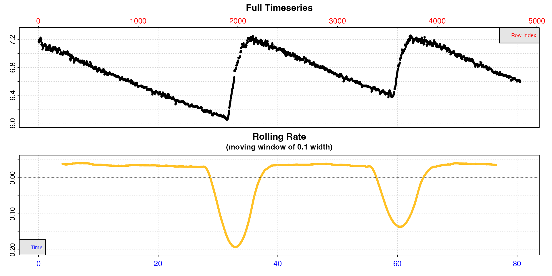

Therefore in the following examples we specify three locations in starts. See the later example for how the starts of regularly spaced replicates are specified.

Changing defaults

By default, if no inputs other than x, starts, and width are entered, the auto_rate default of method = "linear" is applied to all the data in each replicate. This finds the most linear region of a dataset (see vignette("auto_rate")).

auto_rate.int(urchin,
              starts = c(1, 2101, 3901),
              width = 400) |>
  summary()
#> auto_rate.int: The `measure` input is NULL. Calculating rate to the end of the replicate.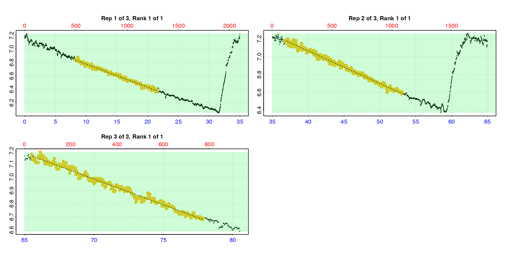

#> 
#> # plot.auto_rate.int # ------------------
#> plot.auto_rate.int: Plotting all rates ...
#> -----------------------------------------
#> 
#> # summary.auto_rate.int # ---------------
#> Summary of all rate results:
#> 
#>    rep rank intercept_b0 slope_b1   rsq density  row endrow  time endtime  oxy endoxy    rate
#> 1:   1    1         7.12  -0.0344 0.988     126  495   1291  8.23    21.5 6.84   6.40 -0.0344
#> 2:   2    1         8.53  -0.0366 0.991     191 2205   3188 36.73    53.1 7.17   6.60 -0.0366
#> 3:   3    1         9.72  -0.0390 0.984     391 3930   4673 65.48    77.9 7.18   6.69 -0.0390
#> -----------------------------------------

Here it performs well in identifying linear regions. However, these inputs mean the flush data is included.

`wait` and `measure`

It is usually a good idea to use the measure input to ensure flushes are excluded and that only relevant data is included in the analysis. We also typically want to exclude some data at the start of a replicate right after the flush, which we can do using wait. All of these are applied in the default units of by = "row". (We also pass legend = TRUE so that the phases are labelled on the plots).

auto_rate.int(urchin,
              starts = c(1, 2101, 3901),
              wait = 300,
              measure = c(1500, 1100, 600),
              width = 400, 
              legend = TRUE) |>
  summary()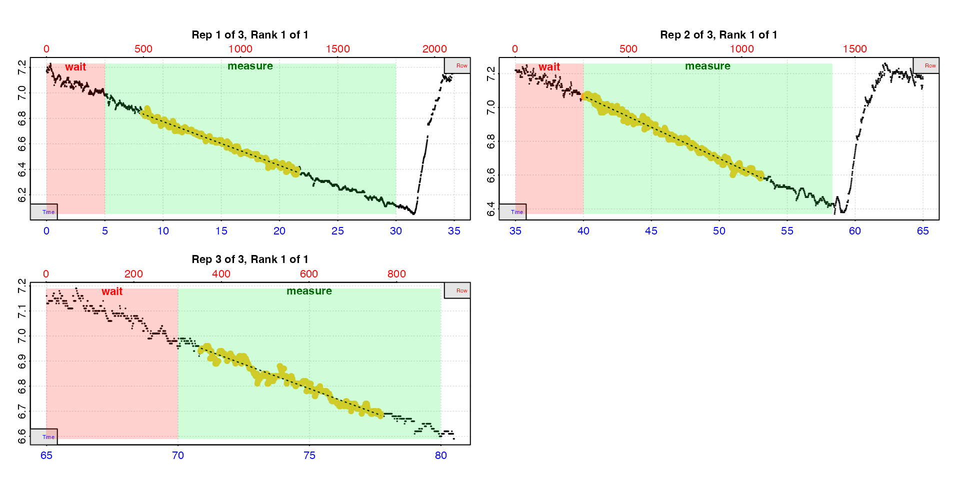

#> 
#> # plot.auto_rate.int # ------------------
#> plot.auto_rate.int: Plotting all rates ...
#> -----------------------------------------
#> 
#> # summary.auto_rate.int # ---------------
#> Summary of all rate results:
#> 
#>    rep rank intercept_b0 slope_b1   rsq density  row endrow  time endtime  oxy endoxy    rate
#> 1:   1    1         7.12  -0.0344 0.988     227  495   1291  8.23    21.5 6.84   6.40 -0.0344
#> 2:   2    1         8.55  -0.0370 0.988     256 2402   3186 40.02    53.1 7.06   6.60 -0.0370
#> 3:   3    1         9.72  -0.0390 0.956     410 4251   4663 70.83    77.7 6.93   6.68 -0.0390
#> -----------------------------------------

Note how the rates (yellow points) do not use the entire measure phase. This is because the auto_rate analysis occurs within the measure phase and the actual lengths of the rate results depends on the method and width. If you want to use the entire measure phase see calc_rate.int().

`n` input

These results show the single top-ranked linear region in each replicate and we can see the rates are fairly consistent. Note there is one result per replicate, with the replicate number in the rep column. The rank column shows ranking of rates within a replicate for the particular method used, and are all 1 here because only one rate has been extracted. You can modify the n input to output more than one rate per replicate. This is what the analysis looks like if it is changed.

auto_rate.int(urchin,
              starts = c(1, 2101, 3901),
              wait = 300,
              measure = c(1500, 1100, 600),
              width = 400, 
              n = 3,
              plot = TRUE,
              legend = TRUE) |>
  summary()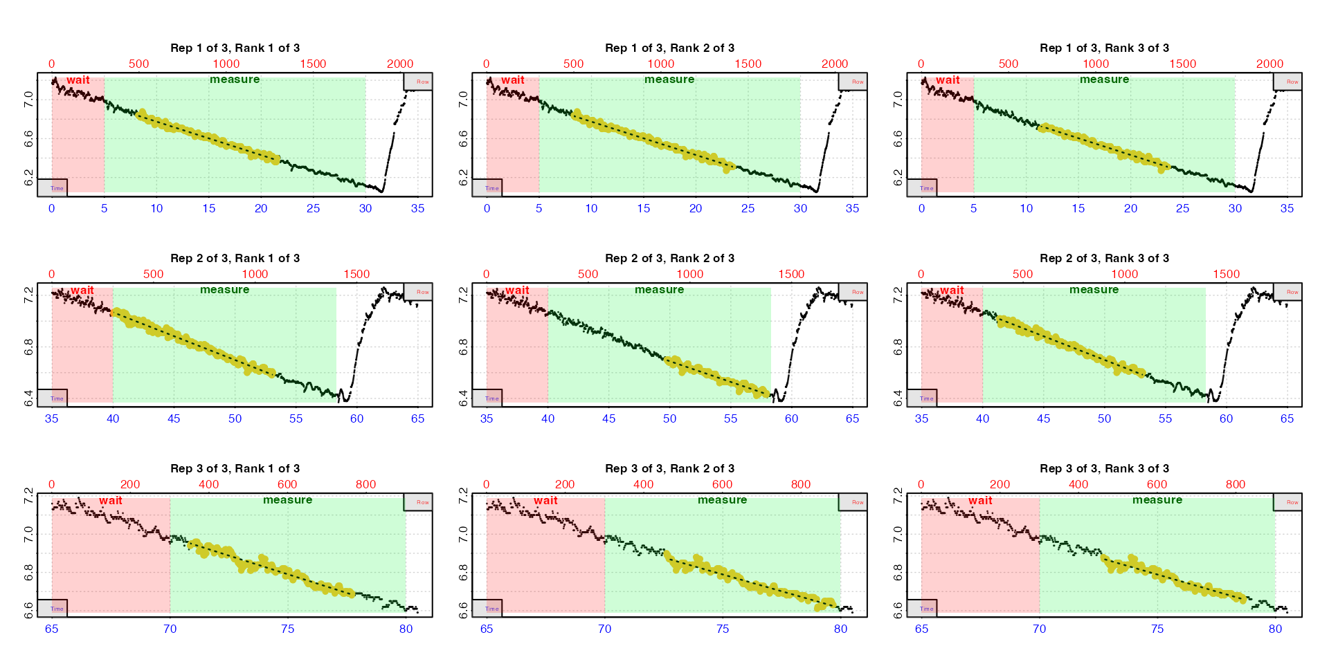

#> 
#> # plot.auto_rate.int # ------------------
#> plot.auto_rate.int: Plotting all rates ...
#> -----------------------------------------
#> 
#> # summary.auto_rate.int # ---------------
#> Summary of all rate results:
#> 
#>    rep rank intercept_b0 slope_b1   rsq density  row endrow  time endtime  oxy endoxy    rate
#> 1:   1    1         7.12  -0.0344 0.988     227  495   1291  8.23    21.5 6.84   6.40 -0.0344
#> 2:   1    2         7.12  -0.0343 0.990     214  499   1412  8.30    23.5 6.84   6.31 -0.0343
#> 3:   1    3         7.12  -0.0345 0.986     213  683   1412 11.37    23.5 6.71   6.31 -0.0345
#> 4:   2    1         8.55  -0.0370 0.988     256 2402   3186 40.02    53.1 7.06   6.60 -0.0370
#> 5:   2    2         8.30  -0.0322 0.958     254 2985   3476 49.73    57.9 6.70   6.43 -0.0322
#> 6:   2    3         8.54  -0.0368 0.985     212 2482   3188 41.35    53.1 7.02   6.60 -0.0368
#> 7:   3    1         9.72  -0.0390 0.956     410 4251   4663 70.83    77.7 6.93   6.68 -0.0390
#> 8:   3    2         9.43  -0.0353 0.955     230 4357   4781 72.60    79.7 6.90   6.63 -0.0353
#> 9:   3    3         9.46  -0.0356 0.942     113 4362   4719 72.68    78.6 6.88   6.66 -0.0356
#> -----------------------------------------

Note the rep and rank columns which keep track of rates.

These results can be passed to adjust_rate and convert_rate for further processing, however consider carefully if you really need to extract more than one rate from each replicate, or if you do be prepared to do a little extra processing of the results (see select_rate()).

Lowest and highest rates

Often in intermittent-flow respirometry we want to get the lowest or highest rates from each replicate, to identify, for example, standard or active metabolic rates. We can do that using the method, width, and by inputs which are passed to auto_rate.

In these examples we use by = "time" selection of regions. This is the lowest rate over a period of 8 minutes from each replicate:

auto_rate.int(urchin,
              starts = c(0, 35, 65),
              wait = 5,
              measure = c(25, 15, 15),
              method = "lowest",
              width = 8,
              by = "time") |>
  summary()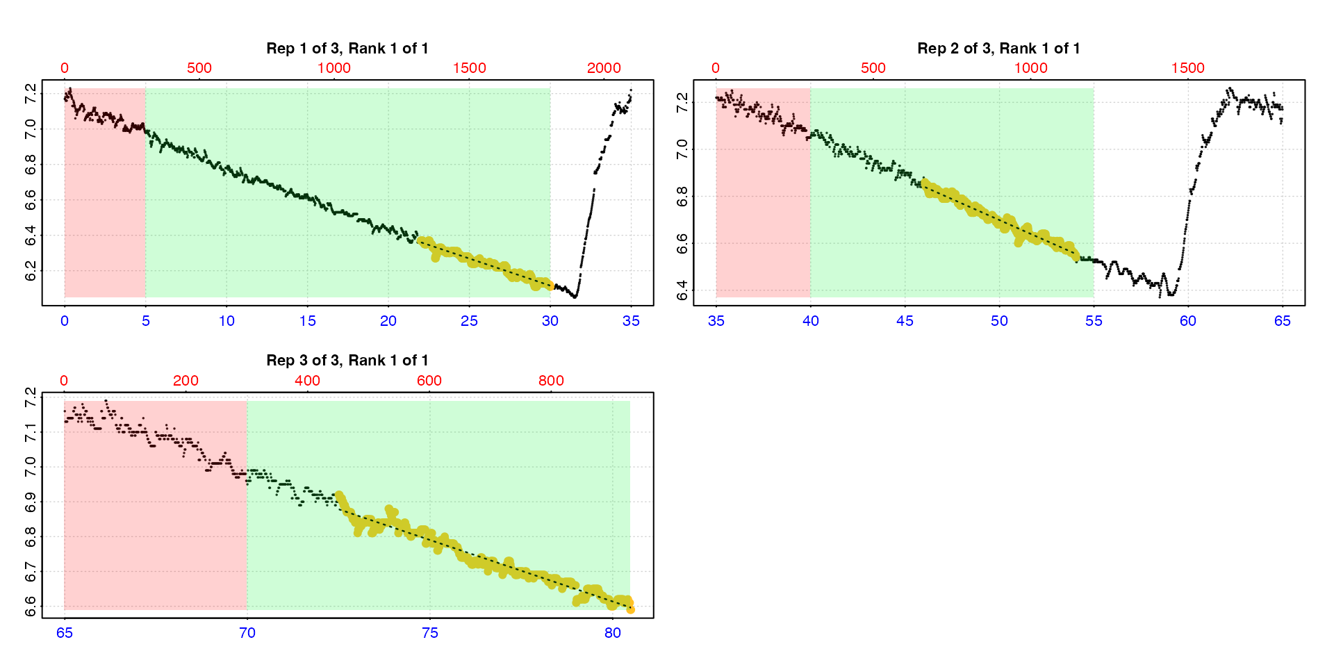

#> 
#> # plot.auto_rate.int # ------------------
#> plot.auto_rate.int: Plotting all rates ...
#> -----------------------------------------
#> 
#> # summary.auto_rate.int # ---------------
#> Summary of all rate results:
#> 
#>    rep rank intercept_b0 slope_b1   rsq density  row endrow time endtime  oxy endoxy    rate
#> 1:   1    1         7.03  -0.0306 0.966      NA 1321   1801 22.0    30.0 6.37   6.11 -0.0306
#> 2:   2    1         8.48  -0.0356 0.969      NA 2764   3244 46.0    54.0 6.86   6.54 -0.0356
#> 3:   3    1         9.44  -0.0353 0.965      NA 4351   4831 72.5    80.5 6.92   6.59 -0.0353
#> -----------------------------------------

This is the highest rate over a period of 8 minutes from each replicate:

auto_rate.int(urchin,
              starts = c(0, 35, 65),
              wait = 5,
              measure = c(25, 15, 15),
              method = "highest",
              width = 8,
              by = "time") |>
  summary()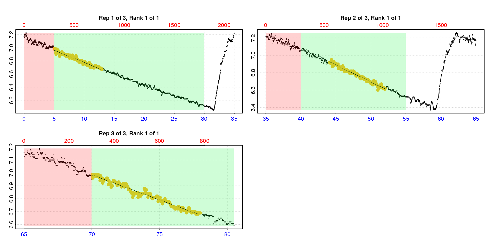

#> 
#> # plot.auto_rate.int # ------------------
#> plot.auto_rate.int: Plotting all rates ...
#> -----------------------------------------
#> 
#> # summary.auto_rate.int # ---------------
#> Summary of all rate results:
#> 
#>    rep rank intercept_b0 slope_b1   rsq density  row endrow time endtime  oxy endoxy    rate
#> 1:   1    1         7.15  -0.0372 0.964      NA  301    781    5      13 6.98   6.67 -0.0372
#> 2:   2    1         8.65  -0.0391 0.974      NA 2644   3124   44      52 6.92   6.62 -0.0391
#> 3:   3    1         9.70  -0.0388 0.969      NA 4202   4682   70      78 6.99   6.69 -0.0388
#> -----------------------------------------

See help("auto_rate") and vignette("auto_rate") for other methods that can be applied.

Regularly spaced replicates

For intermittent-flow experiments where the replicates are regularly spaced you do not have to specify the start location of every single one in starts, but can instead enter a single value indicating the interval in rows or a time duration between each one starting at the first row of the input data.

Specify regular replicate structure

The zeb_intermittent.rd example dataset uses a regular replicate structure of 9 minutes measure and 2 minutes flush (660 rows total) for most of its length. See help("zeb_intermittent.rd") for exact locations, but essentially after a background control and a single replicate of 14 minutes this structure is maintained until the ending background recording. Therefore to use this option we need to use subset_data() (or other methods in R to subset data) to extract only the regular replicates, and pipe the result to auto_rate.int. We use starts to specify that replicates cycle at 660 rows, impose a wait phase of 2 minutes, a measure phase of 7 minutes to exclude the flush, and use the other inputs to extract the lowest rate of 3 minutes duration.

zeb_all <- zeb_intermittent.rd |>
  
  # Inspect the data
  inspect() |>
  
  # Subset regular replicates from larger dataset
  subset_data(from = 5840,
              to = 75139,
              by = "row",
              quiet = TRUE) |>
  
  # Use auto_rate.int to get lowest 3 minute rate from each replicate, 
  # plotting first 3 and last 3 (using 'pos')
  auto_rate.int(starts = 660,
                wait = 120,
                measure = 420,
                width = 180,
                method = "lowest",
                plot = TRUE,
                pos = c(1:3, 103:105))

Here we use the pos input which is passed to plot to select the first and last three replicates for plotting to check everything looks okay. This is only for illustration here. In an actual experiment we strongly recommend every replicate rate result be examined visually. Up to 20 results at a time can be plotted using the pos input. See Plot section below for further details.

View summary

Each replicate result is saved in the $summary element of the output, or we can use summary().

summary(zeb_all)
#> 
#> # summary.auto_rate.int # ---------------
#> Summary of all rate results:
#> 
#>      rep rank intercept_b0 slope_b1   rsq density   row endrow  time endtime  oxy endoxy     rate
#>   1:   1    1         48.5 -0.00707 0.992      NA   157    336  5996    6175 6.10   4.81 -0.00707
#>   2:   2    1         33.1 -0.00411 0.957      NA  1021   1200  6860    7039 5.00   4.10 -0.00411
#>   3:   3    1         47.4 -0.00559 0.966      NA  1681   1860  7520    7699 5.44   4.35 -0.00559
#>   4:   4    1         38.1 -0.00392 0.977      NA  2202   2381  8041    8220 6.59   5.89 -0.00392
#>   5:   5    1         36.0 -0.00336 0.958      NA  2967   3146  8806    8985 6.40   5.74 -0.00336
#>  ---                                                                                             
#> 101: 101    1        157.0 -0.00207 0.927      NA 66271  66450 72110   72289 7.36   7.02 -0.00207
#> 102: 102    1        163.1 -0.00214 0.921      NA 67021  67200 72860   73039 7.20   6.85 -0.00214
#> 103: 103    1        162.9 -0.00212 0.933      NA 67677  67856 73516   73695 7.22   6.82 -0.00212
#> 104: 104    1        170.0 -0.00220 0.941      NA 68209  68388 74048   74227 7.48   7.10 -0.00220
#> 105: 105    1        155.5 -0.00198 0.920      NA 68917  69096 74756   74935 7.39   6.99 -0.00198
#> -----------------------------------------

This object is now ready to be passed to adjust_rate() and convert_rate(). Final rate selection can be handled using select_rate() after conversion. See vignette("select_rate") and vignette("intermittent_long") for examples.

Plot

If plot = TRUE, a plot is produced of each replicate rate result on a grid up to a total of 20. By default this is the first 20 (i.e. pos = 1:20). Others can be selected by modifying the pos input, either in the main function call or when calling plot() on output objects.

plot(zeb_all, pos = 50:69)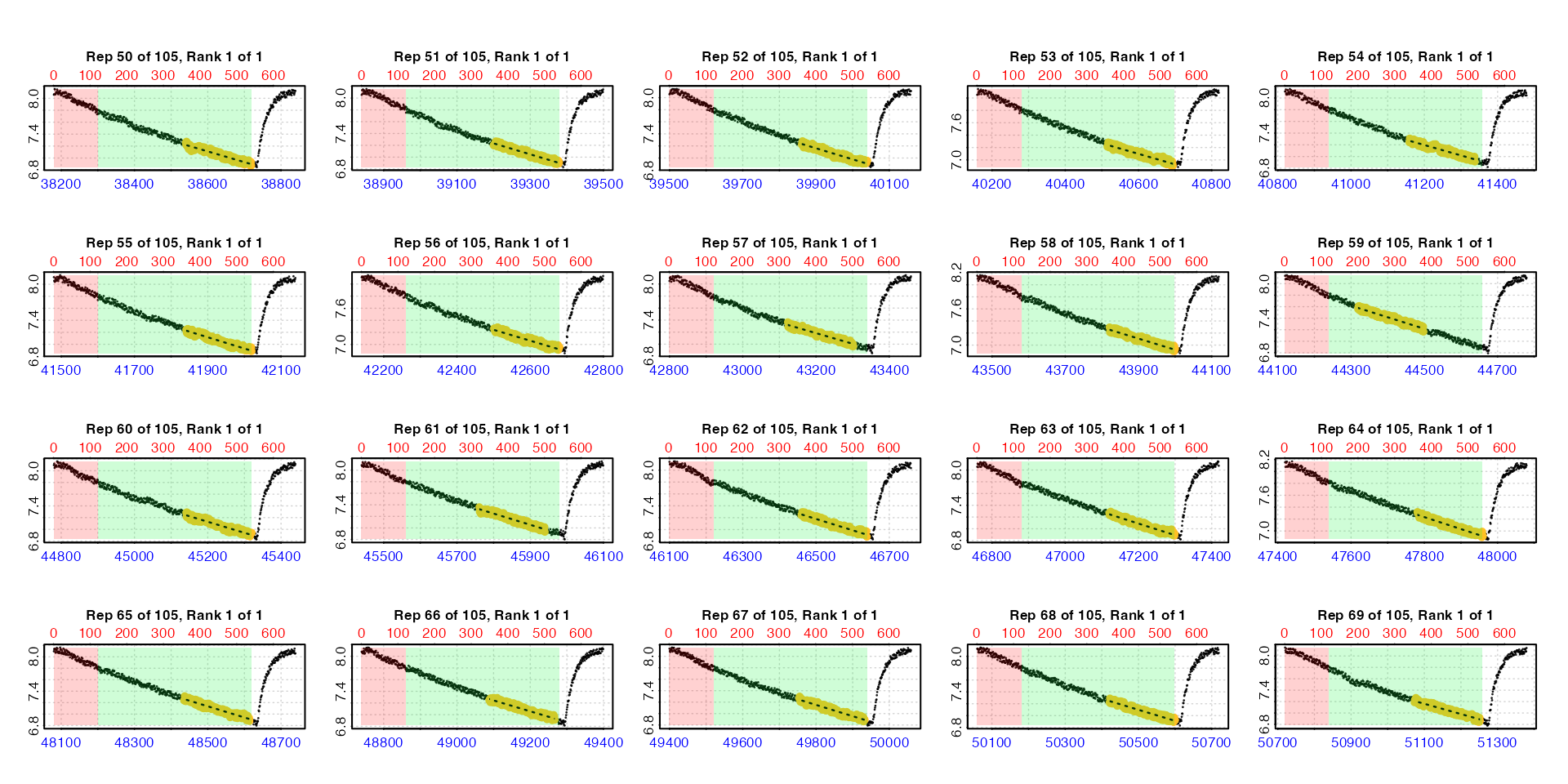

There are three ways in which these auto_rate.int results can be plotted, selected using the type input in either the main function call or when calling plot() on output objects. For all plots, the bottom blue time axis shows the time values of the original larger dataset, whilst the upper red row axis shows the rows of the replicate subset.

`type = "rep"`

The default is type = "rep" in which each replicate is plotted individually with the rate region highlighted. The rate data is the yellow points, the red shaded region is the wait phase, and the green shaded region the measure phase.

urch <- auto_rate.int(urchin,
                      starts = c(1, 2101, 3901),
                      wait = 300,
                      measure = c(1500, 1100, 600),
                      width = 400, 
                      plot = TRUE,
                      type = "rep",
                      legend = TRUE)

`type = "full"`

Entering type = "full" will show each replicate rate highlighted in the context of the entire dataset.

auto_rate.int(urchin,
              starts = c(1, 2101, 3901),
              wait = 300,
              measure = c(1500, 1100, 600),
              width = 400, 
              plot = TRUE,
              type = "full")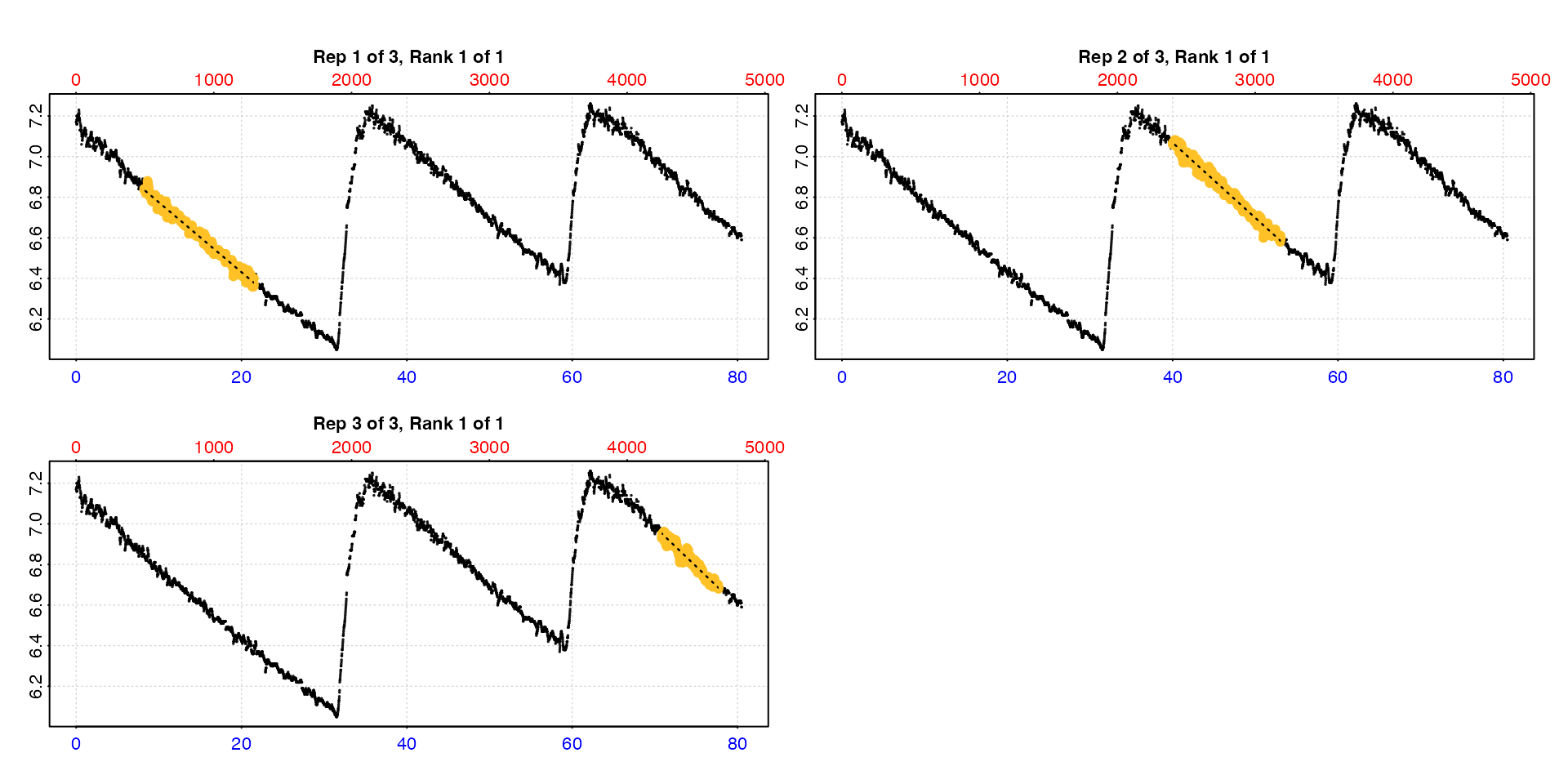

Note this may be of limited use when the dataset is large.

plot(zeb_all, type = "full", pos = 50)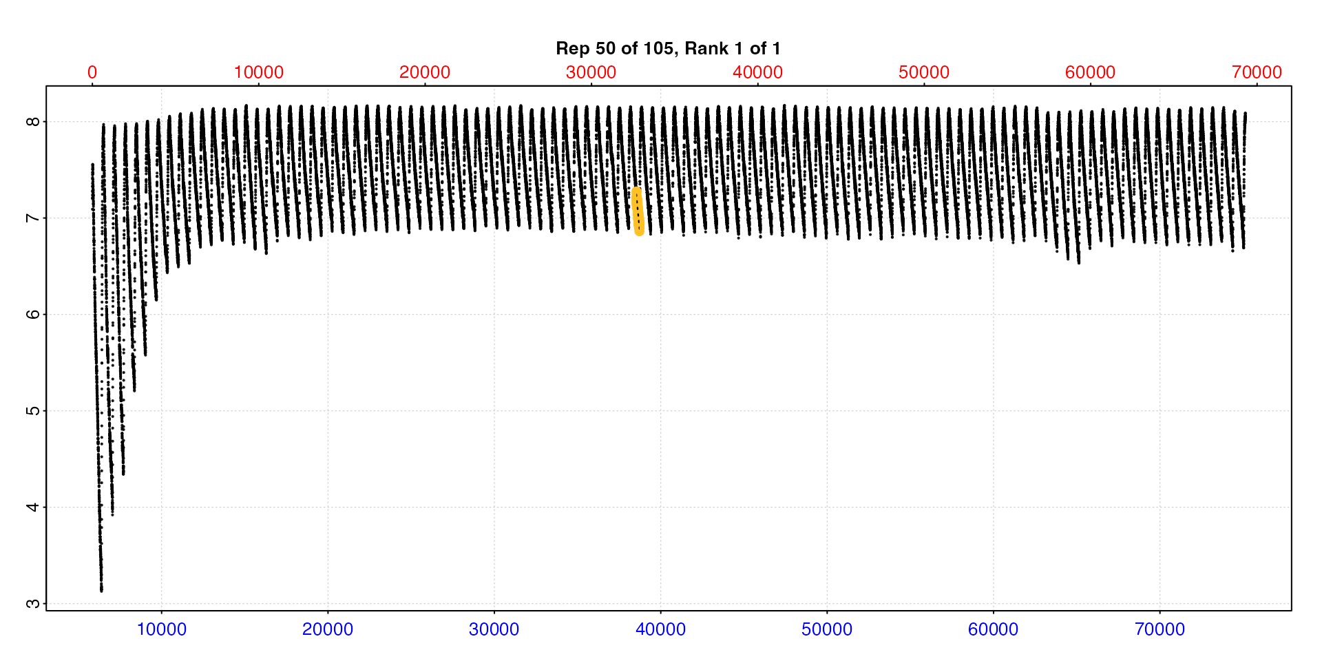

`type = "ar"`

Lastly, the auto_rate result (as found in the $results element of the output) for each individual row of the summary table can be plotted using type = "ar" and the pos input. Note these plots show only the measure phase of the data and the rate result from within it.

plot(zeb_all, type = "ar", pos = 50)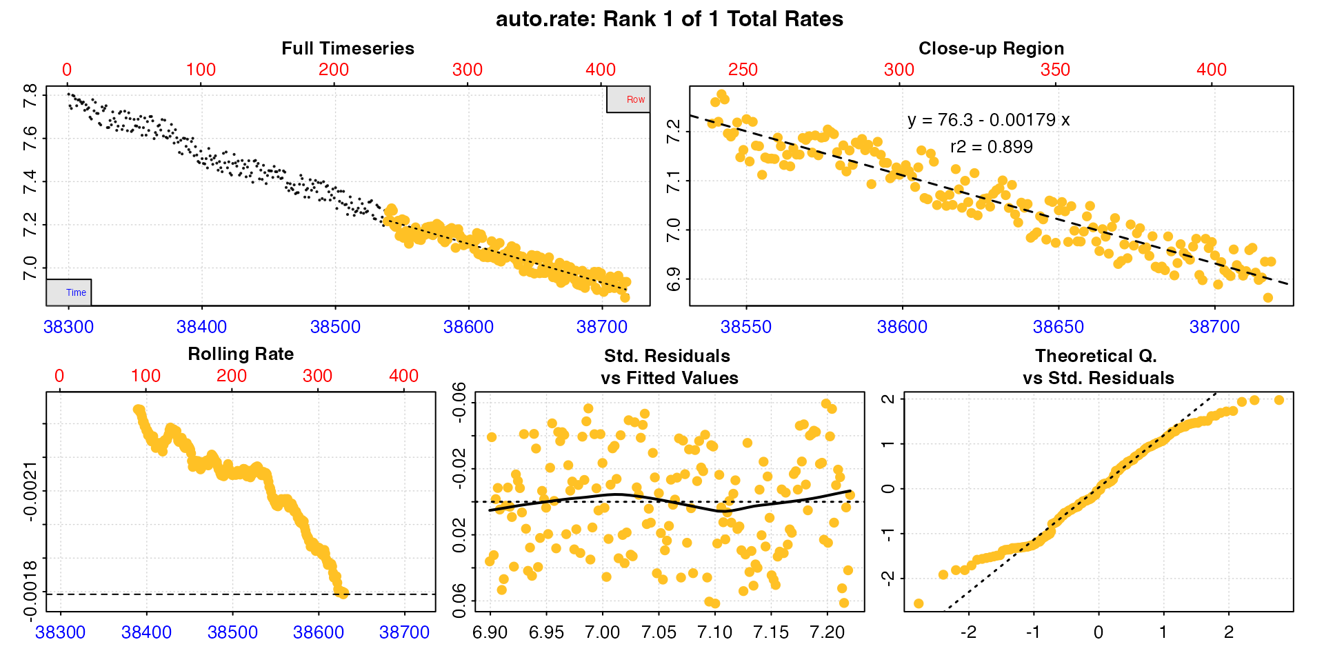

The pos input here can also be of multiple replicates but this will produce multiple individual plots.

Additional plotting options

legend can be used to show labels (default is FALSE). quiet suppresses console output. Additional plotting parameters can also be passed to adjust margins, axis label rotation, etc. See here.

S3 generic methods

As well as plot, saved auto_rate.int objects work with the generic S3 methods print, summary, and mean

`print`

This simply prints a single summary row rate result to the console, by default the first one. The pos input can be used to print others.

print(zeb_all)
#> 
#> # print.auto_rate.int # -----------------
#> 
#> Replicate 1 of 105, Rank 1 of 1:
#> Rate: -0.00707 
#> 
#> To see other results use 'pos' input. 
#> To see full results use summary().
#> -----------------------------------------
print(zeb_all, pos = 50)
#> 
#> # print.auto_rate.int # -----------------
#> 
#> Replicate 50 of 105, Rank 1 of 1:
#> Rate: -0.00179 
#> 
#> To see other results use 'pos' input. 
#> To see full results use summary().
#> -----------------------------------------

`summary`

This prints the summary table to the console which contains linear model coefficients and other metadata for each replicate rate. The pos input can be used to select which replicates ($rep column) to include.

summary(zeb_all)
#> 
#> # summary.auto_rate.int # ---------------
#> Summary of all rate results:
#> 
#>      rep rank intercept_b0 slope_b1   rsq density   row endrow  time endtime  oxy endoxy     rate
#>   1:   1    1         48.5 -0.00707 0.992      NA   157    336  5996    6175 6.10   4.81 -0.00707
#>   2:   2    1         33.1 -0.00411 0.957      NA  1021   1200  6860    7039 5.00   4.10 -0.00411
#>   3:   3    1         47.4 -0.00559 0.966      NA  1681   1860  7520    7699 5.44   4.35 -0.00559
#>   4:   4    1         38.1 -0.00392 0.977      NA  2202   2381  8041    8220 6.59   5.89 -0.00392
#>   5:   5    1         36.0 -0.00336 0.958      NA  2967   3146  8806    8985 6.40   5.74 -0.00336
#>  ---                                                                                             
#> 101: 101    1        157.0 -0.00207 0.927      NA 66271  66450 72110   72289 7.36   7.02 -0.00207
#> 102: 102    1        163.1 -0.00214 0.921      NA 67021  67200 72860   73039 7.20   6.85 -0.00214
#> 103: 103    1        162.9 -0.00212 0.933      NA 67677  67856 73516   73695 7.22   6.82 -0.00212
#> 104: 104    1        170.0 -0.00220 0.941      NA 68209  68388 74048   74227 7.48   7.10 -0.00220
#> 105: 105    1        155.5 -0.00198 0.920      NA 68917  69096 74756   74935 7.39   6.99 -0.00198
#> -----------------------------------------
summary(zeb_all, pos = 1:4)
#> 
#> # summary.auto_rate.int # ---------------
#> Summary of results from entered 'pos' row(s):
#> 
#>    rep rank intercept_b0 slope_b1   rsq density  row endrow time endtime  oxy endoxy     rate
#> 1:   1    1         48.5 -0.00707 0.992      NA  157    336 5996    6175 6.10   4.81 -0.00707
#> 2:   2    1         33.1 -0.00411 0.957      NA 1021   1200 6860    7039 5.00   4.10 -0.00411
#> 3:   3    1         47.4 -0.00559 0.966      NA 1681   1860 7520    7699 5.44   4.35 -0.00559
#> 4:   4    1         38.1 -0.00392 0.977      NA 2202   2381 8041    8220 6.59   5.89 -0.00392
#> -----------------------------------------

export = TRUE can be used to export the summary table as a data frame, or those rows selected using pos

zeb_exp <- summary(zeb_all, 
                   pos = 1:4, 
                   export = TRUE)

zeb_exp
#>    rep rank intercept_b0 slope_b1   rsq density  row endrow time endtime  oxy endoxy     rate
#> 1:   1    1         48.5 -0.00707 0.992      NA  157    336 5996    6175 6.10   4.81 -0.00707
#> 2:   2    1         33.1 -0.00411 0.957      NA 1021   1200 6860    7039 5.00   4.10 -0.00411
#> 3:   3    1         47.4 -0.00559 0.966      NA 1681   1860 7520    7699 5.44   4.35 -0.00559
#> 4:   4    1         38.1 -0.00392 0.977      NA 2202   2381 8041    8220 6.59   5.89 -0.00392

`mean`

This averages all replicate rates in the $rate column, or those selected using pos. The result can be saved as a value by using export = TRUE.

zeb_mean <- mean(zeb_all, pos = 1:4, export = TRUE)
#> 
#> # mean.auto_rate.int # ------------------
#> Mean of rate results from entered 'pos' rows:
#> 
#> Mean of 4 rates:
#> [1] -0.00517
#> -----------------------------------------
zeb_mean
#> [1] -0.00517

This could be passed as a numeric value to later functions such as convert_rate(), although it is usually better to do this kind of result filtering after conversion.