inspect() is a data exploration and preparation function that visualises
respirometry data and checks it for errors that may affect the use of further
functions in respR. It also subsets specified columns into a new list
object that can be used in subsequent functions, reducing the need for
additional inputs. Note, use of inspect to prepare data for the subsequent
functions is optional. Functions in respR can accept regular R data
objects including data frames, data tables, tibbles, vectors, etc. It is a
quality control and exploratory step to help users view and prepare their
data prior to analysis.
Arguments
- x
data.frame. Any object of class
data.frame(incl.data.table,tibble, etc.). Should contain paired numeric values of time and oxygen.- time
integer or string. Defaults to
1. Specifies the column of the Time data as either a column number or the name.- oxygen
integer or string, or vector of either. Defaults to
2. Specifies the column(s) of the Oxygen data as either a vector of column numbers or names.- width
numeric, 0.01 to 1. Defaults to
0.1. Width used in the rolling regression plot as proportion of total length of data.- plot
logical. Defaults to
TRUE. Plots the data. Iftimeand singleoxygencolumns selected, plots timeseries data, plus plot of rolling rate. If multipleoxygencolumns, plots all timeseries data only.- add.data
integer or string. Defaults to
NULL. Specifies the column number or name of an optional additional data source that will be plotted in blue alongside the full oxygen timeseries.- ...
Allows additional plotting controls to be passed, such as
legend = FALSE,rate.rev = FALSEandpos. A differentwidthcan also be passed inplot()commands on output objects.
Value
Output is a list object of class inspect, with a $dataframe
containing the specified time and oxygen columns, inputs, and metadata
which can be passed to calc_rate() or auto_rate() to determine
rates. If there are failed checks or warnings, the row locations of the
potentially problematic data can be found in $locs.
Details
Given an input data frame, x, the function scans the specified time and
oxygen columns for the following issues. Columns are specified by using the
column number (e.g. time = 1), or by name (e.g. time = "Time.Hrs"). If
time and oxygen are left NULL the default of time = 1, oxygen = 2 is
applied.
Check for numeric data
respR requires data be in the form of paired values of numeric time and
oxygen. All columns are checked that they contain numeric data before any
other checks are performed. If any of the inspected columns do not contain
numeric data the remaining checks for that column are skipped, and the
function exits returning NULL, printing the summary of the checks. No plot
is produced. Only when all inspected columns pass this numeric check can the
resulting output object be saved and passed to other respR functions.
Other checks
The time column is checked for missing (NA/NaN) values, positive and
negative infinite values (Inf/-Inf), that values are sequential, that there
are no duplicate times, and that it is numerically evenly-spaced. Oxygen
columns are checked for missing (NA/NaN) and infinite values (Inf/-Inf).
See Failed Checks section for what it means for analyses if these checks
result in warnings. If the output is assigned, the specified time and
oxygen columns are extracted and saved to a list object for use in later
functions such as calc_rate() and auto_rate(). A plot is also
produced.
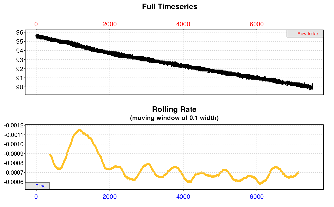
Plot
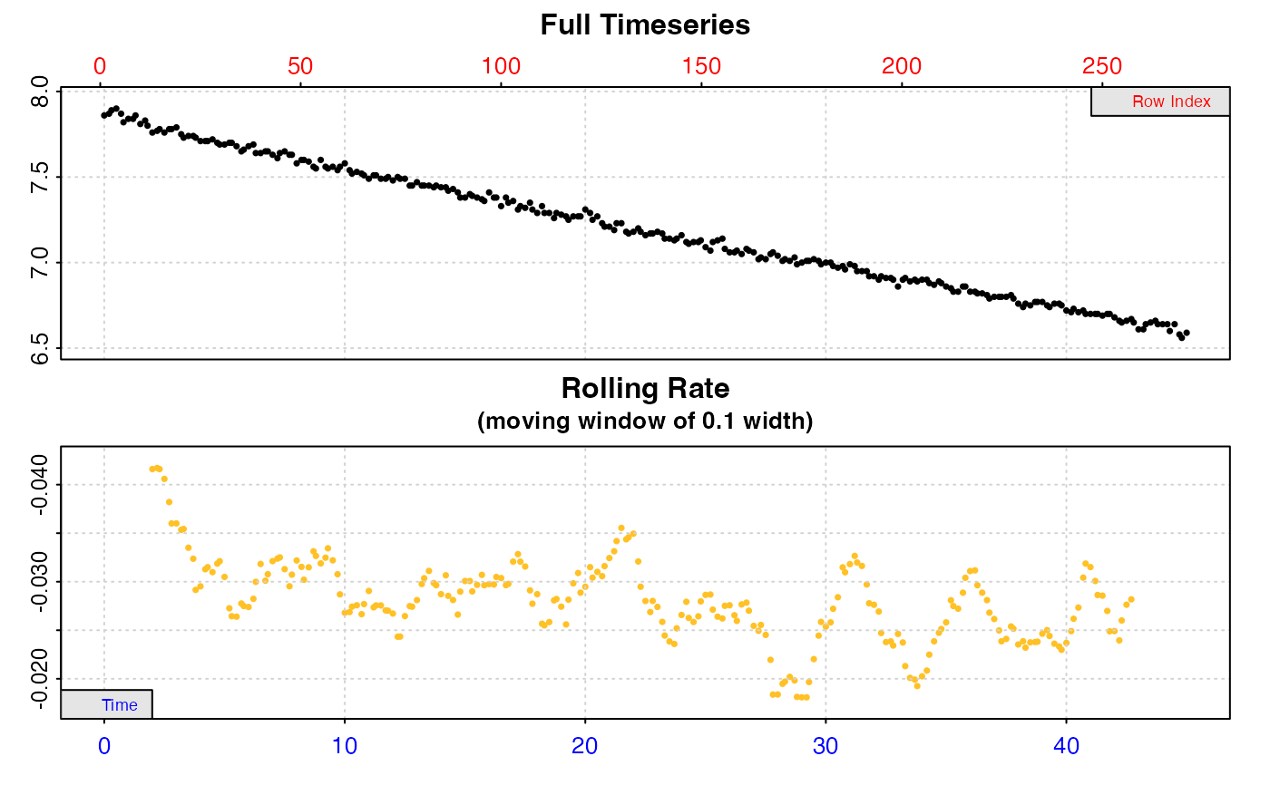
If plot = TRUE (the default), a plot of the oxygen timeseries is produced
in the upper panel. In addition, a rolling regression plot in the lower panel
shows the rate of change in oxygen across a rolling window specified using
the width operator (default is width = 0.1, or 10% of the entire
dataset). This plot provides a quick visual inspection of how the rate varies
over the course of the experiment. Regions of stable and consistent rates can
be identified on this plot as flat or level areas. This plot is for
exploratory purposes only; later functions allow rate to be calculated over
specific regions. Each individual rate value is plotted against the centre of
the time window used to calculate it.
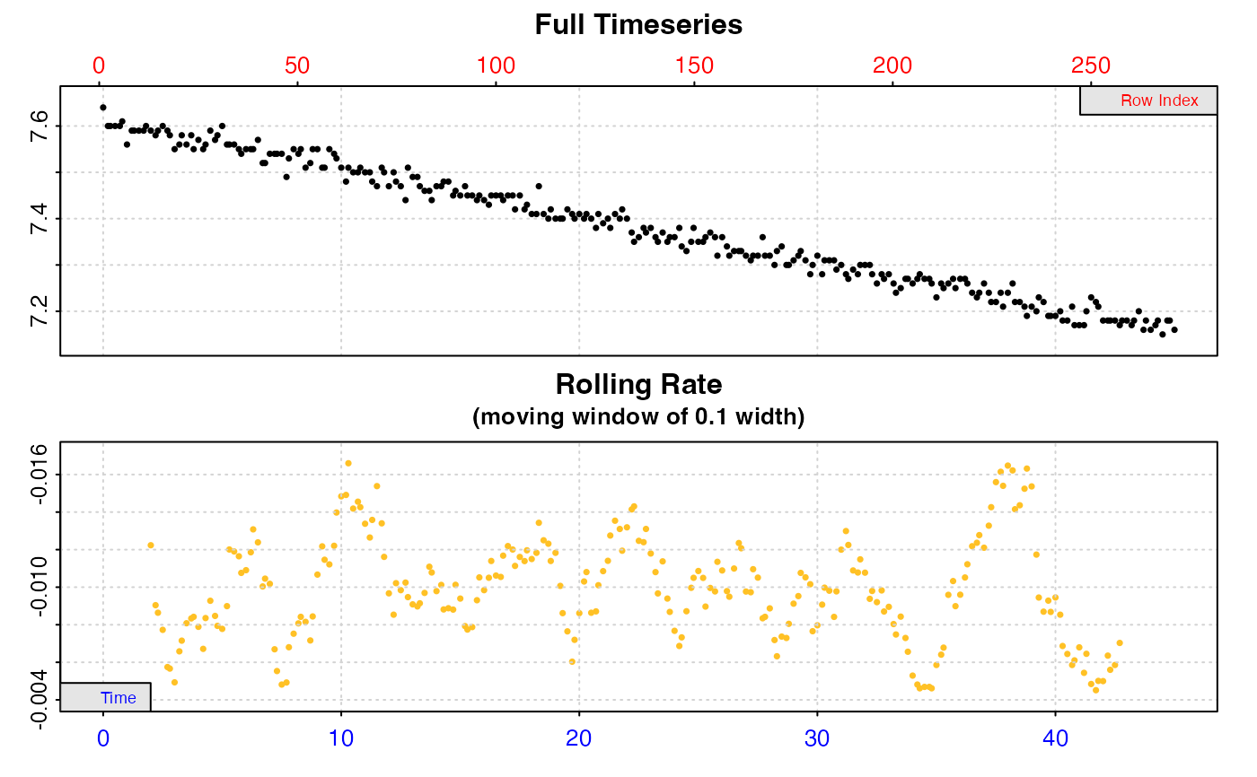
Note: Since respR is primarily used to examine oxygen consumption,
the oxygen rate plot is by default plotted on a reverse y-axis. In respR
oxygen uptake rates are negative since they represent a negative slope of
oxygen against time. In these plots the axis is reversed so that higher
uptake rates (i.e. more negative) will be higher on these plots. If you are
interested instead in oxygen production rates, which are positive, the
rate.rev = FALSE input can be passed in either the inspect call, or when
using plot() on the output object. In this case, the rate values will be
plotted numerically, and higher oxygen production rates will be higher on
the plot.
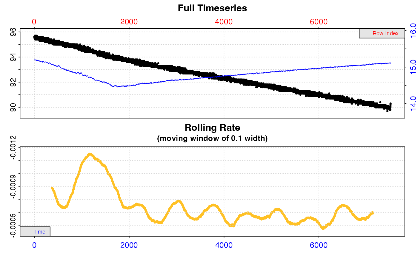
Plot an additional data source
Using the add.data input an additional data source, for example
temperature, can be plotted alongside the oxygen timeseries. This should be
either a column number (e.g. add.data = 3) or name (e.g. add.data = "Temperature") indicating a column in the input x data frame sharing the
same time data. None of the data checks are performed on this column; it is
simply to give a basic visual aid in the plot to, for example, help decide if
regions of the data should be used or not used because this parameter was
variable. Values are saved in the output as a vector under $add.data. It is
plotted in blue on a separate y-axis on the main timeseries plot. It is not
plotted if multiple oxygen columns are inspected. See examples.
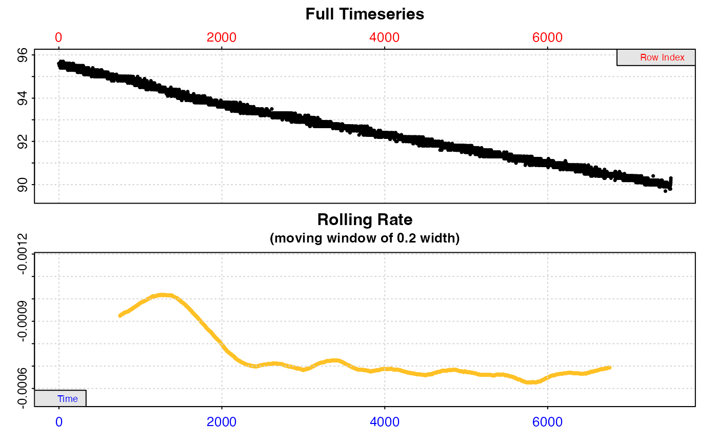
Additional plotting options
A different width value can be passed to see how it affects estimation of
the rolling rate. If axis labels obscure parts of the plot they can be
suppressed using legend = FALSE. If multiple columns have been inspected,
the pos input can be used to examine each time~oxygen dataset. If axis
labels (particularly y-axis) are difficult to read, las = 2 can be passed
to make axis labels horizontal, and oma (outer margins, default oma = c(0.4, 1, 1.5, 0.4)) or mai (inner margins, default mai = c(0.3, 0.15, 0.35, 0.15)) can be used to adjust plot margins. See examples.
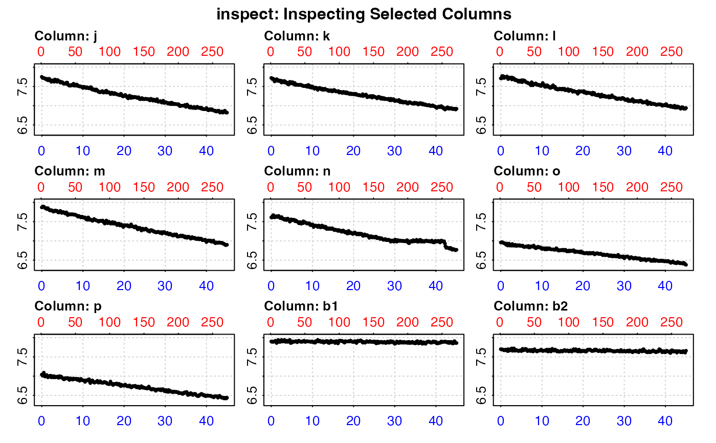
Multiple Columns of Oxygen Data
For a quick overview of larger datasets, multiple oxygen columns can be
inspected for errors and plotted by using the oxygen input to select
multiple columns. These must share the same time column. In this case, data
checks are performed, with a plot of each oxygen time series, but no rolling
rate plot is produced. All data are plotted on the same axis range of both
time and oxygen (total range of data). This is chiefly exploratory
functionality to allow for a quick overview of a dataset, and it should be
noted that while the output inspect object will contain all columns in its
$dataframe element, subsequent functions in respR (calc_rate,
auto_rate, etc.) will by default only use the first two columns (time,
and the first specified oxygen column). To analyse multiple columns and
determine rates, best practice is to inspect and assign each time-oxygen
column pair as separate inspect objects. See Examples.
Flowthrough Respirometry Data
For flowthrough respirometry data, see the specialised inspect.ft()
function.
Failed Checks
The most important data check in inspect is that all data columns are
numeric. If any column fails this check, the function skips the remaining
checks for that column, the function exits returning NULL, and no output
object or plot is produced.
The other failed check that requires action is the check for infinite values
(Inf/-Inf). Some oxygen sensing systems add these in error when
interference or data dropouts occur. Infinite values will cause problems when
it comes to calculating rates, so need to be removed. If found, locations of
these are printed and can be found in the output object under $locs. Note,
these values are not plotted, so special note should be taken of the warnings
and console printout.
The remaining data checks in inspect are mainly exploratory and help
diagnose and flag potential issues with the data that might affect rate
calculations. For instance, long experiments may have had sensor dropouts the
user is unaware of. Some might not be major issues. For instance, an uneven
time warning can result from using decimalised minutes, which is a completely
valid time metric, but happens to be numerically unevenly spaced. As an
additional check, if uneven time is found, the minimum and maximum intervals
in the time data are in the console output, so a user can see immediately if
there are large gaps in the data.
If some of these checks produce warnings, it should generally not hinder
analysis of the data. respR has been coded to rely on linear regressions on
exact data values, and not make assumptions about data spacing or order.
Therefore issues such as missing or NA/NaN values, duplicate or
non-sequential time values, or uneven time spacing should not cause any
erroneous rate results, as long as they do not occur over large regions of
the data. inspect however outputs locations (row numbers) of where these
issues occur (located in the $locs element of the output), allowing users
to amend them before analysis. We would strongly recommend that to be
completely confident in any results from analysis of such data, and avoid
obscure errors, these issues be addressed before proceeding.
S3 Generic Functions
Saved output objects can be used in the generic S3 functions plot(),
print() and summary().
More
For additional help, documentation, vignettes, and more visit the respR
website at https://januarharianto.github.io/respR/
Examples
# \donttest{
## By default, assumes time is col 1 and oxygen col2:
inspect(sardine.rd)
#> inspect: Applying column default of 'time = 1'
#> inspect: Applying column default of 'oxygen = 2'
#> inspect: No issues detected while inspecting data frame.
#>
#> # print.inspect # -----------------------
#> Time Oxygen
#> numeric pass pass
#> Inf/-Inf pass pass
#> NA/NaN pass pass
#> sequential pass -
#> duplicated pass -
#> evenly-spaced pass -
#>
#> -----------------------------------------
 ## Instead, specify time and oxygen columns as either number or name
inspect(sardine.rd, time = 1, oxygen = 2)
#> inspect: No issues detected while inspecting data frame.
#>
#> # print.inspect # -----------------------
#> Time Oxygen
#> numeric pass pass
#> Inf/-Inf pass pass
#> NA/NaN pass pass
#> sequential pass -
#> duplicated pass -
#> evenly-spaced pass -
#>
#> -----------------------------------------
inspect(urchins.rd, time = "time.min", oxygen = "a")
#> Warning: inspect: Time values are not evenly-spaced (numerically).
#> inspect: Data issues detected. For more information use print().
#>
#> # print.inspect # -----------------------
#> time.min a
#> numeric pass pass
#> Inf/-Inf pass pass
#> NA/NaN pass pass
#> sequential pass -
#> duplicated pass -
#> evenly-spaced WARN -
#>
#> Uneven Time data locations (first 20 shown) in column: time.min
#> [1] 1 2 3 4 5 6 7 8 9 10 11 12 13 14 15 16 17 18 19 20
#> Minimum and Maximum intervals in uneven Time data:
#> [1] 0.1 0.2
#> -----------------------------------------
## Instead, specify time and oxygen columns as either number or name
inspect(sardine.rd, time = 1, oxygen = 2)
#> inspect: No issues detected while inspecting data frame.
#>
#> # print.inspect # -----------------------
#> Time Oxygen
#> numeric pass pass
#> Inf/-Inf pass pass
#> NA/NaN pass pass
#> sequential pass -
#> duplicated pass -
#> evenly-spaced pass -
#>
#> -----------------------------------------
inspect(urchins.rd, time = "time.min", oxygen = "a")
#> Warning: inspect: Time values are not evenly-spaced (numerically).
#> inspect: Data issues detected. For more information use print().
#>
#> # print.inspect # -----------------------
#> time.min a
#> numeric pass pass
#> Inf/-Inf pass pass
#> NA/NaN pass pass
#> sequential pass -
#> duplicated pass -
#> evenly-spaced WARN -
#>
#> Uneven Time data locations (first 20 shown) in column: time.min
#> [1] 1 2 3 4 5 6 7 8 9 10 11 12 13 14 15 16 17 18 19 20
#> Minimum and Maximum intervals in uneven Time data:
#> [1] 0.1 0.2
#> -----------------------------------------
 ## Use add.data input to plot an additional data type
## (this column is not checked)
inspect(sardine.rd, time = 1, oxygen = 2, add.data = 3)
#> inspect: No issues detected while inspecting data frame.
#>
#> # print.inspect # -----------------------
#> Time Oxygen
#> numeric pass pass
#> Inf/-Inf pass pass
#> NA/NaN pass pass
#> sequential pass -
#> duplicated pass -
#> evenly-spaced pass -
#>
#> -----------------------------------------
## Use add.data input to plot an additional data type
## (this column is not checked)
inspect(sardine.rd, time = 1, oxygen = 2, add.data = 3)
#> inspect: No issues detected while inspecting data frame.
#>
#> # print.inspect # -----------------------
#> Time Oxygen
#> numeric pass pass
#> Inf/-Inf pass pass
#> NA/NaN pass pass
#> sequential pass -
#> duplicated pass -
#> evenly-spaced pass -
#>
#> -----------------------------------------
 ## Adjust the width of the rolling rate plot:
inspect(sardine.rd, 1, 2, width = 0.2)
#> inspect: No issues detected while inspecting data frame.
#>
#> # print.inspect # -----------------------
#> Time Oxygen
#> numeric pass pass
#> Inf/-Inf pass pass
#> NA/NaN pass pass
#> sequential pass -
#> duplicated pass -
#> evenly-spaced pass -
#>
#> -----------------------------------------
## Adjust the width of the rolling rate plot:
inspect(sardine.rd, 1, 2, width = 0.2)
#> inspect: No issues detected while inspecting data frame.
#>
#> # print.inspect # -----------------------
#> Time Oxygen
#> numeric pass pass
#> Inf/-Inf pass pass
#> NA/NaN pass pass
#> sequential pass -
#> duplicated pass -
#> evenly-spaced pass -
#>
#> -----------------------------------------
 ## Inspect specific columns in multicolumn datasets:
inspect(urchins.rd, time = 1, oxygen = 4)
#> Warning: inspect: Time values are not evenly-spaced (numerically).
#> inspect: Data issues detected. For more information use print().
#>
#> # print.inspect # -----------------------
#> time.min c
#> numeric pass pass
#> Inf/-Inf pass pass
#> NA/NaN pass pass
#> sequential pass -
#> duplicated pass -
#> evenly-spaced WARN -
#>
#> Uneven Time data locations (first 20 shown) in column: time.min
#> [1] 1 2 3 4 5 6 7 8 9 10 11 12 13 14 15 16 17 18 19 20
#> Minimum and Maximum intervals in uneven Time data:
#> [1] 0.1 0.2
#> -----------------------------------------
## Inspect specific columns in multicolumn datasets:
inspect(urchins.rd, time = 1, oxygen = 4)
#> Warning: inspect: Time values are not evenly-spaced (numerically).
#> inspect: Data issues detected. For more information use print().
#>
#> # print.inspect # -----------------------
#> time.min c
#> numeric pass pass
#> Inf/-Inf pass pass
#> NA/NaN pass pass
#> sequential pass -
#> duplicated pass -
#> evenly-spaced WARN -
#>
#> Uneven Time data locations (first 20 shown) in column: time.min
#> [1] 1 2 3 4 5 6 7 8 9 10 11 12 13 14 15 16 17 18 19 20
#> Minimum and Maximum intervals in uneven Time data:
#> [1] 0.1 0.2
#> -----------------------------------------
 ## Inspect multiple columns for a quick overview
## of a large dataset:
inspect(urchins.rd, time = 1, oxygen = c(11:19))
#> inspect: Multiple 'oxygen' columns selected. Note that subsequent functions in respR will by default use first oxygen column only.
#> Warning: inspect: Time values are not evenly-spaced (numerically).
#> inspect: Data issues detected. For more information use print().
#>
#> # print.inspect # -----------------------
#> time.min j k l m n o p b1 b2
#> numeric pass pass pass pass pass pass pass pass pass pass
#> Inf/-Inf pass pass pass pass pass pass pass pass pass pass
#> NA/NaN pass pass pass pass pass pass pass pass pass pass
#> sequential pass - - - - - - - - -
#> duplicated pass - - - - - - - - -
#> evenly-spaced WARN - - - - - - - - -
#>
#> Uneven Time data locations (first 20 shown) in column: time.min
#> [1] 1 2 3 4 5 6 7 8 9 10 11 12 13 14 15 16 17 18 19 20
#> Minimum and Maximum intervals in uneven Time data:
#> [1] 0.1 0.2
#> -----------------------------------------
## Inspect multiple columns for a quick overview
## of a large dataset:
inspect(urchins.rd, time = 1, oxygen = c(11:19))
#> inspect: Multiple 'oxygen' columns selected. Note that subsequent functions in respR will by default use first oxygen column only.
#> Warning: inspect: Time values are not evenly-spaced (numerically).
#> inspect: Data issues detected. For more information use print().
#>
#> # print.inspect # -----------------------
#> time.min j k l m n o p b1 b2
#> numeric pass pass pass pass pass pass pass pass pass pass
#> Inf/-Inf pass pass pass pass pass pass pass pass pass pass
#> NA/NaN pass pass pass pass pass pass pass pass pass pass
#> sequential pass - - - - - - - - -
#> duplicated pass - - - - - - - - -
#> evenly-spaced WARN - - - - - - - - -
#>
#> Uneven Time data locations (first 20 shown) in column: time.min
#> [1] 1 2 3 4 5 6 7 8 9 10 11 12 13 14 15 16 17 18 19 20
#> Minimum and Maximum intervals in uneven Time data:
#> [1] 0.1 0.2
#> -----------------------------------------
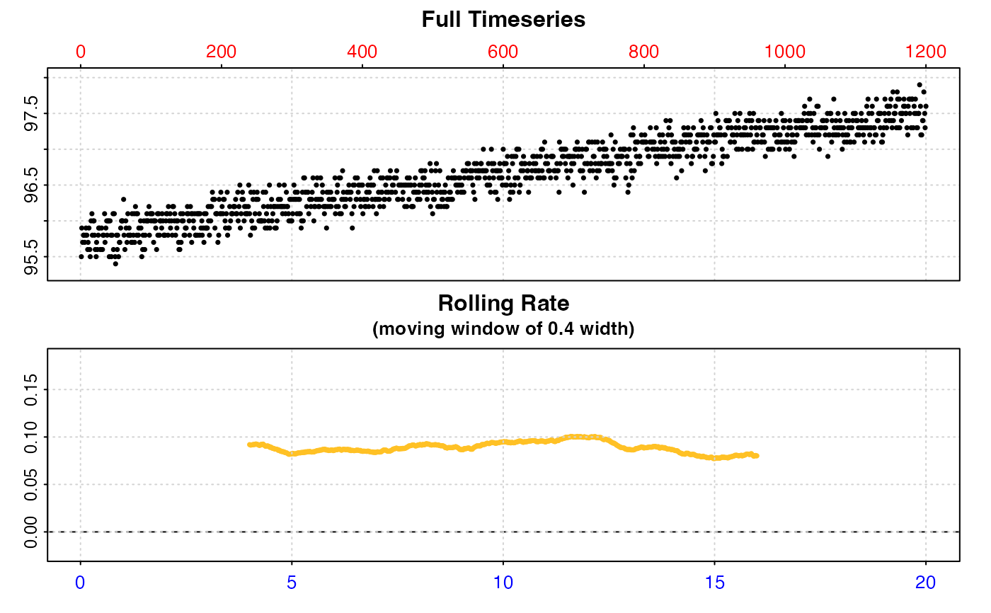
 ## Inspect oxygen production data, use a width that gives
## a better rolling rate, and use extra plotting options to
## suppress legend, and ensure rates are plotted not reversed:
inspect(algae.rd, time = 1, oxygen = 2, width = 0.4,
legend = FALSE, rate.rev = FALSE)
#> Warning: inspect: Time values are not evenly-spaced (numerically).
#> inspect: Data issues detected. For more information use print().
#>
#> # print.inspect # -----------------------
#> Time Oxygen
#> numeric pass pass
#> Inf/-Inf pass pass
#> NA/NaN pass pass
#> sequential pass -
#> duplicated pass -
#> evenly-spaced WARN -
#>
#> Uneven Time data locations (first 20 shown) in column: Time
#> [1] 1 2 3 4 5 6 7 8 9 10 11 12 13 14 15 16 17 18 19 20
#> Minimum and Maximum intervals in uneven Time data:
#> [1] 0.01 0.02
#> -----------------------------------------
## Inspect oxygen production data, use a width that gives
## a better rolling rate, and use extra plotting options to
## suppress legend, and ensure rates are plotted not reversed:
inspect(algae.rd, time = 1, oxygen = 2, width = 0.4,
legend = FALSE, rate.rev = FALSE)
#> Warning: inspect: Time values are not evenly-spaced (numerically).
#> inspect: Data issues detected. For more information use print().
#>
#> # print.inspect # -----------------------
#> Time Oxygen
#> numeric pass pass
#> Inf/-Inf pass pass
#> NA/NaN pass pass
#> sequential pass -
#> duplicated pass -
#> evenly-spaced WARN -
#>
#> Uneven Time data locations (first 20 shown) in column: Time
#> [1] 1 2 3 4 5 6 7 8 9 10 11 12 13 14 15 16 17 18 19 20
#> Minimum and Maximum intervals in uneven Time data:
#> [1] 0.01 0.02
#> -----------------------------------------
 ## Pass additional plotting inputs to override defaults and
## allow better y-axis label visibility
inspect(sardine.rd, time = 1, oxygen = 2,
las = 1, mai = c(0.3, 0.35, 0.35, 0.15))
#> inspect: No issues detected while inspecting data frame.
#>
#> # print.inspect # -----------------------
#> Time Oxygen
#> numeric pass pass
#> Inf/-Inf pass pass
#> NA/NaN pass pass
#> sequential pass -
#> duplicated pass -
#> evenly-spaced pass -
#>
#> -----------------------------------------
## Pass additional plotting inputs to override defaults and
## allow better y-axis label visibility
inspect(sardine.rd, time = 1, oxygen = 2,
las = 1, mai = c(0.3, 0.35, 0.35, 0.15))
#> inspect: No issues detected while inspecting data frame.
#>
#> # print.inspect # -----------------------
#> Time Oxygen
#> numeric pass pass
#> Inf/-Inf pass pass
#> NA/NaN pass pass
#> sequential pass -
#> duplicated pass -
#> evenly-spaced pass -
#>
#> -----------------------------------------
 # }
# }