Calculate rate of change in oxygen over time

Calculates rate of oxygen uptake or production from respirometry data. A rate can be determined over the whole dataset, or on subsets of the data using the from and to inputs to specify data regions in terms of oxygen or time units or row numbers of the input data. Multiple rates can be extracted from the same dataset by using these inputs to enter vectors of paired values in the appropriate metric. See Examples.

calc_rate(x, from = NULL, to = NULL, by = "time", plot = TRUE, ...)

Arguments

x: object of class inspect or data.frame. This is the timeseries of paired values of oxygen against time from which to calculate rates.
from: numeric value or vector. Defaults to NULL. The start of the region(s) over which you want to calculate the rate in the units specified in by. If a vector, each value must have a paired value in to.
to: numeric value or vector. Defaults to NULL. The end of the region(s) over which you want to calculate the rate in the units specified in by. If a vector, each value must have a paired value in from.
by: string. "time", "row", or "oxygen". Defaults to "time". This is the method used to subset the data region between from and to.
plot: logical. Defaults to TRUE. Plot the results.
...: Allows additional plotting controls to be passed, such as pos, panel, and quiet = TRUE.

Value

Output is a list object of class calc_rate containing input parameters and data, various summary data, metadata, linear models, and the primary output of interest $rate, which can be background adjusted in adjust_rate or converted to units in convert_rate.

Details

The function calculates rates by fitting a linear model of oxygen against time, with the slope of this regression being the rate. There are no units involved in calc_rate. This is a deliberate decision. The units of oxygen concentration and time will be specified later in convert_rate() when rates are converted to specific output units.

For continuous data recordings, it is recommended a data.frame containing the data be prepared via inspect(), and entered as the x input. For data not prepared like this, x can be a 2-column data.frame containing numeric values of time (col 1) and oxygen (col 2). If multiple columns are found in either an inspect or data frame input, only the first two columns are used.

Specifying regions

For calculating rates over specific regions of the data, the from and to inputs in the by units of "time" (the default), "oxygen", or "row". The from and to inputs do not need to be precise; the function will use the closest values found.

Multiple regions can be examined within the same dataset by entering from and to as vectors of paired values to specify different regions. In this case, $rate in the output will be a vector of multiple rates with each result corresponding to the position of the paired from and to inputs. If from and to are NULL (the default), the rate is determined over the entire dataset.

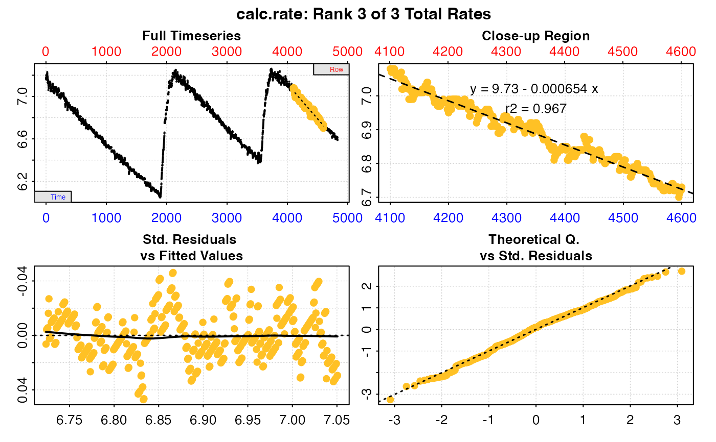
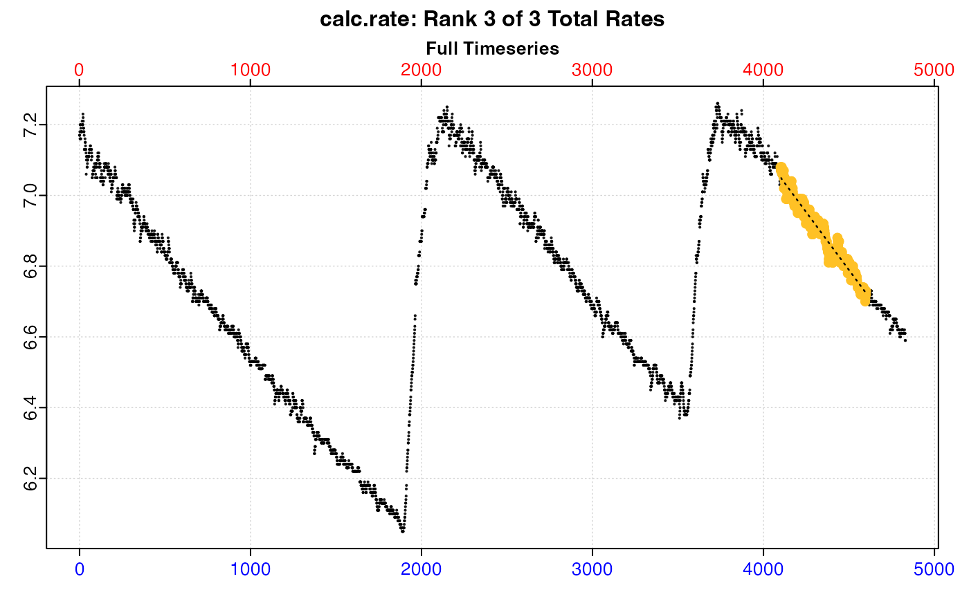
Plot

A plot is produced (provided plot = TRUE) showing the original data timeseries of oxygen against time (bottom blue axis) and row index (top red axis), with the region specified via the from and to inputs highlighted. Second panel is a close-up of the rate region with linear model coefficients. Third and fourth panels are summary plots of fit and residuals.

Additional plotting options

If multiple rates have been calculated, by default the first (pos = 1) is plotted. Others can be plotted by changing the pos input either in the main function call, or by plotting the output, e.g. plot(object, pos = 2). In addition, each sub-panel can be examined individually by using the panel input, e.g. plot(object, panel = 2).

Console output messages can be suppressed using quiet = TRUE. If axis labels (particularly y-axis) are difficult to read, las = 2 can be passed to make axis labels horizontal, and oma (outer margins, default oma = c(0.4, 1, 1.5, 0.4)), and mai (inner margins, default mai = c(0.3, 0.15, 0.35, 0.15)) used to adjust plot margins.

S3 Generic Functions

Saved output objects can be used in the generic S3 functions print(), summary(), and mean().

print(): prints a single result, by default the first rate. Others can be printed by passing the pos input. e.g. print(x, pos = 2)
summary(): prints summary table of all results and metadata, or those specified by the pos input. e.g. summary(x, pos = 1:5). The summary can be exported as a separate dataframe by passing export = TRUE.
mean(): calculates the mean of all rates, or those specified by the pos input. e.g. mean(x, pos = 1:5) The mean can be exported as a separate value by passing export = TRUE.

For additional help, documentation, vignettes, and more visit the respR website at https://januarharianto.github.io/respR/

Examples

# Subset by 'time' (the default)
inspect(sardine.rd, time = 1, oxygen = 2, plot = FALSE) %>%
  calc_rate(from = 200, to = 1800)
#> inspect: No issues detected while inspecting data frame.
#> 
#> # print.inspect # -----------------------
#>                 Time Oxygen
#> numeric         pass   pass
#> Inf/-Inf        pass   pass
#> NA/NaN          pass   pass
#> sequential      pass      -
#> duplicated      pass      -
#> evenly-spaced   pass      -
#> 
#> -----------------------------------------

#> 
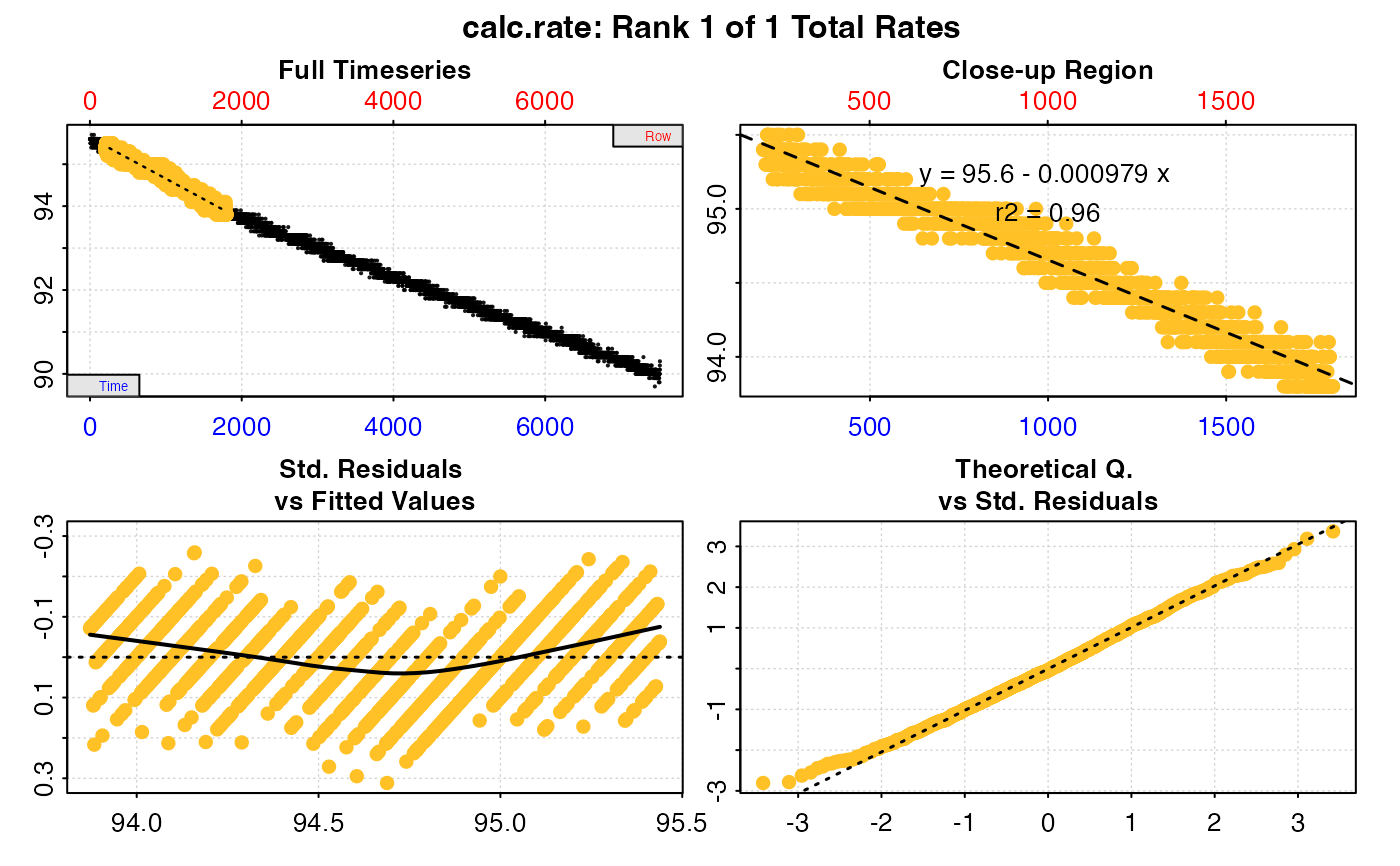#> # print.calc_rate # ---------------------
#> Rank 1 of 1 rates:
#> Rate: -0.0009793698 
#> 
#> To see full results use summary().
#> -----------------------------------------

# Subset by oxygen
inspect(sardine.rd, time = 1, oxygen = 2, plot = FALSE) %>%
  calc_rate(94, 91, by = "oxygen")
#> inspect: No issues detected while inspecting data frame.
#> 
#> # print.inspect # -----------------------
#>                 Time Oxygen
#> numeric         pass   pass
#> Inf/-Inf        pass   pass
#> NA/NaN          pass   pass
#> sequential      pass      -
#> duplicated      pass      -
#> evenly-spaced   pass      -
#> 
#> -----------------------------------------

#> 
#> # print.calc_rate # ---------------------
#> Rank 1 of 1 rates:
#> Rate: -0.0006892677 
#> 
#> To see full results use summary().
#> -----------------------------------------

# Subset by row
inspect(sardine.rd, time = 1, oxygen = 2, plot = FALSE) %>%
  calc_rate(1000, 2000, by = "row")
#> inspect: No issues detected while inspecting data frame.
#> 
#> # print.inspect # -----------------------
#>                 Time Oxygen
#> numeric         pass   pass
#> Inf/-Inf        pass   pass
#> NA/NaN          pass   pass
#> sequential      pass      -
#> duplicated      pass      -
#> evenly-spaced   pass      -
#> 
#> -----------------------------------------

#> 
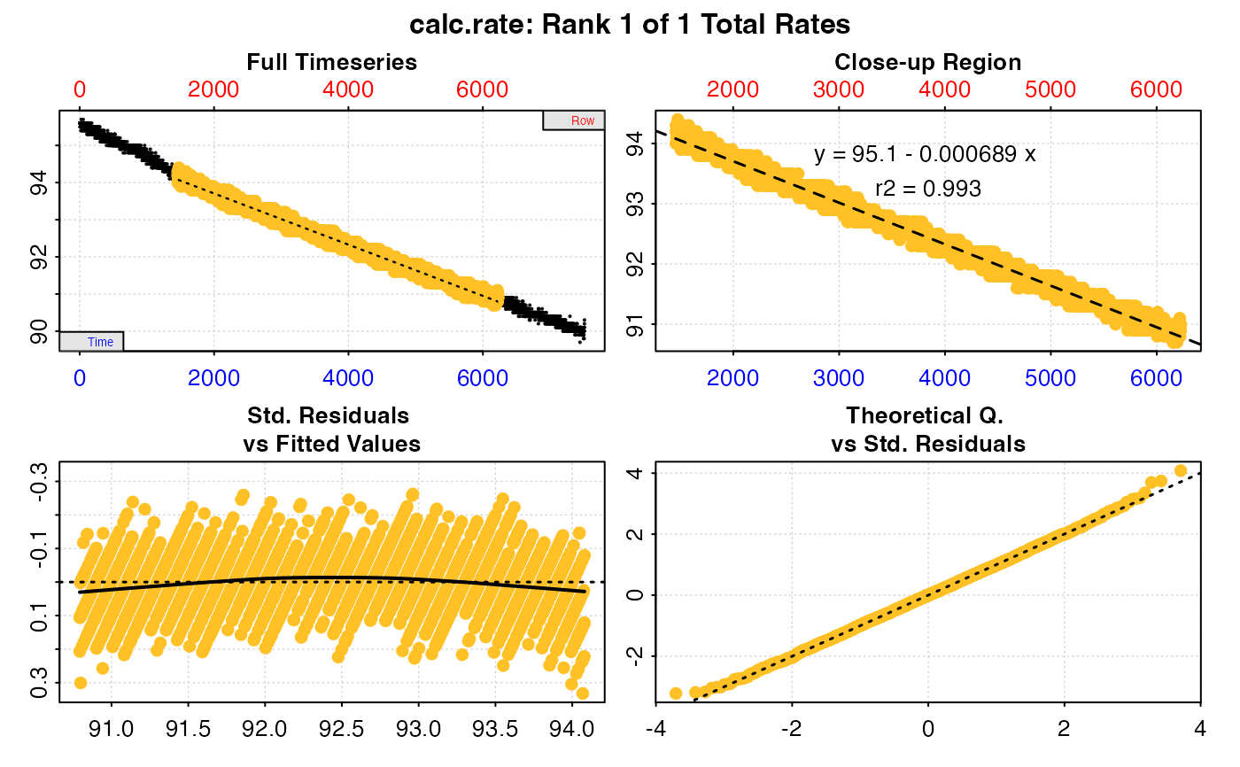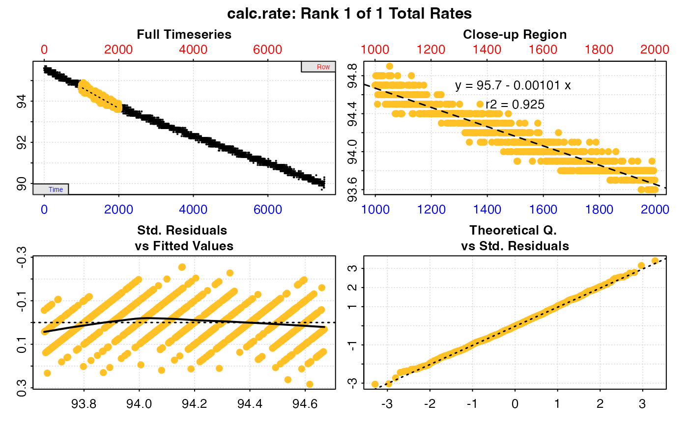#> # print.calc_rate # ---------------------
#> Rank 1 of 1 rates:
#> Rate: -0.001012827 
#> 
#> To see full results use summary().
#> -----------------------------------------

# Use a data frame input, and calculate rate from multiple regions by
# using a vector in the 'from' and 'to' inputs
x <- calc_rate(intermittent.rd,
               from = c(200,2300,4100),
               to = c(1800,3200,4600),
               by = 'time',
               plot = FALSE)
# Print and summary of results
print(x)
#> 
#> # print.calc_rate # ---------------------
#> Rank 1 of 3 rates:
#> Rate: -0.0005734109 
#> 
#> To see other results use 'pos' input. 
#> To see full results use summary().
#> -----------------------------------------
summary(x)
#> 
#> # summary.calc_rate # -------------------
#> Summary of all rate results:
#> 
#>    rep rank intercept_b0      slope_b1   rsq  row endrow time endtime  oxy endoxy   rate.2pt          rate
#> 1:  NA    1     7.127202 -0.0005734109 0.995  201   1801  200    1800 7.05   6.11 -0.0005875 -0.0005734109
#> 2:  NA    2     8.528274 -0.0006097325 0.990 2301   3201 2300    3200 7.12   6.58 -0.0006000 -0.0006097325
#> 3:  NA    3     9.731918 -0.0006539752 0.967 4101   4601 4100    4600 7.08   6.73 -0.0007000 -0.0006539752
#> -----------------------------------------
# Plot the third of these results
plot(x, pos = 3)
#> 
#> # plot.calc_rate # ----------------------
#> plot.calc_rate: Plotting rate from position 3 of 3 ...

#> -----------------------------------------
# Plot only the timeseries plot and hide the legend
plot(x, pos = 3, panel = 1, legend = FALSE)
#> 
#> # plot.calc_rate # ----------------------
#> plot.calc_rate: Plotting rate from position 3 of 3 ...

#> -----------------------------------------