auto_rate: Automatic detection of metabolic rates

Introduction

In respirometry, we want to report oxygen uptake or production rates from experimentally important stages or that represent behavioural or physiological states. These include:

the most linear, that is most consistent or monotonic rates observed, often most representative of routine metabolism
the lowest rates observed, often most representative of standard, resting, basal or maintenance metabolism
the highest rates observed, representative of active or maximum metabolic rates

Identifying and extracting these rates from large datasets is difficult, and if selected visually, subject to observer bias and lack of objectivity. Methods such as fitting multiple, fixed-width linear regressions over an entire dataset to identify regions of lowest or highest slopes (i.e. rates) is computationally intensive, and slopes found via this method highly sensitive to the width chosen, especially if the specimen’s metabolic rate changes rapidly or the data is noisy.

Here we detail auto_rate(), a function that uses machine learning techniques to automatically detect the most linear regions of a dataset. This allows an investigator to extract rates in a statistically robust, objective manner. It can also extract and order highest and lowest rates, or return an unordered rolling rate across the whole dataset.

In this vignette we detail how auto_rate works, and how it can be used to extract rates from respirometry data. Importantly, auto_rate has been optimised to be extremely fast. Other methods on large datasets can take minutes, hours or even days to run. auto_rate can reduce this wait by orders of magnitude, fitting tens of thousands of regressions and detecting linear regions in seconds.

Overview

This illustrates the main processes involved in auto_rate:

auto_rate works by performing an optimised rolling regression on the dataset of a specified width. For the linear method, a kernel density estimate is performed on the rolling regression output, and the kernel bandwidth used to re-sample linear regions of the data for re-analysis. For other methods, the results are filtered, ordered, or returned unordered.

Rolling linear regression

The function auto_rate uses a novel method of combining rolling regression and kernel density estimate algorithms to detect patterns in time series data. The rolling regression runs all possible ordinary least-squares (OLS) linear regressions $(y = \beta_0 + \beta_1 X + \epsilon)$ of a fixed sample width across the dataset, and is expressed as: $y_t(n) = X_t(n) \beta (n) + \epsilon_t(n), \ t = n,\ ...,\ T$ where $T$ is the total length of the dataset, $n$ is the window of width $n < T$ , $y_t(n)$ is the vector of observations (e.g. oxygen concentration), $X_t(n)$ is the matrix of explanatory variables, $\beta (n)$ is a vector of regression parameters and $\epsilon_t(n)$ is a vector of error terms. Thus, a total of $(T - n) + 1$ number of overlapping regressions are fit.

Methods

auto_rate has several methods to process, order or filter the rolling regression results.

`method = "linear"`

This method uses kernel density estimation (KDE) to automatically identify linear regions of the dataset.

First, we take advantage of the key assumption that linear sections of a data series are reflected by stable parameters across the rolling estimates, a property that is often applied in financial statistics to evaluate model stability and make forward predictions on time-series data (see Zivot and Wang 2006). We use kernel density estimation (KDE) techniques, often applied in various inference procedures such as machine learning, pattern recognition and computer vision, to automatically aggregate stable (i.e. linear) segments as they naturally form one or more local maxima (“modes”) in the probability density estimate.

KDE requires no assumption that the data is from a parametric family, and learns the shape of the density automatically without supervision. KDE can be expressed as: $\hat{f}(x) = \frac{1}{nh^d}\sum_{i = 1}^{n} K \left(\frac{x - X_i}{h} \right)$ where $f$ is the density function from an unknown distribution $P$ for $X_1,...,X_n$ , $K$ is the kernel function and $h$ is the optimal smoothing bandwidth. The smoothing bandwidth is computed using the solve-the-equation plug-in method (Sheather et al. 1996, Sheather and Jones 1991) which works well with multimodal or non-normal densities (Raykar and Duraiswami 2006).

We then use $h$ to select all values in the rolling regression output that match the range of values around each mode ( $\theta_n$ ) of the KDE (i.e. $\theta_n \pm h$ ). These rolling estimates are grouped and ranked by size, and the upper and lower bounds of the data windows they represent are used to re-select the linear segment of the original data series. The rolling estimates are then discarded while the detected data segments are analysed using linear regression.

The output will contain only the regressions identified as coming from linear regions of the data, ranked by order of the KDE density analysis. This is present in the $summary component of the output as $density. Under this method, the width input is used as a starting seed value, but the resulting regressions may be of any width.

When this method might be applied

This method could be applied to virtually any respirometry data when you are looking for linear regions where rates are stable, consistent and representative rates for the behavioural or physiological state of the specimen. This could be a routine metabolic rate, standard or basal metabolic rate, or in the case of an animal under constant exercise a consistent active metabolic rate.

`method = "lowest"`

Every regression of the specified width across the timeseries is calculated, then ordered using absolute rate values from lowest to highest. This option can only be used when rates all have the same sign, and it essentially ignores the sign. Rates will be ordered from lowest to highest in the $summary table by absolute value regardless of if they are positive or negative.

When this method might be applied

When you are looking for the lowest rates across a specific time or row window, representative of resting, basal or standard metabolic rates.

`method = "highest"`

Every regression of the specified width across the timeseries is calculated, then ordered using absolute rate values from highest to lowest. This option can only be used when rates all have the same sign, and it essentially ignores the sign. Rates will be ordered from highest to lowest in the $summary table by absolute value regardless of if they are positive or negative.

When this method might be applied

When you are looking for the highest rates across a specific time or row window, representative of maximum or active metabolic rates.

`method = "minimum"`, `method = "maximum"`

These methods are strictly numerical and take full account of the sign of the rate. In respR oxygen uptake rates are negative since they represent a negative slope of oxygen against time, and oxygen production rates are positive.

Every regression of the specified width across the entire timeseries is calculated, then ordered using numerical rate values from minimum to maximum for the minimum method, or vice versa for maximum. Generally this method should only be used when rates are a mix of oxygen consumption and production rates, such as when positive rates may result from regressions fit over flush periods in intermittent-flow respirometry.

When these methods might be applied

Generally, for most analyses where high or low rates are of interest the highest or lowest methods should be used instead. However, when rates are a mix of negative and positive and you want the highest or lowest these can be used, but note they order by numerical value; the highest oxygen uptake rates will be most minimum.

`method = "rolling"`

This method returns all regressions of the specified width in sequential order across the dataset. All results are returned in the summary table.

When this method might be applied

This method can be applied when you want to extract a rolling rate of a specified width for further analyses. Alternatively, if you don’t want to rely on the "linear" selection or other methods but want to filter and select the results according to various criteria using select_rate(). See vignette("select_rate").

`method = "interval"`

Multiple, successive, non-overlapping regressions of the specified ‘width’ are extracted from the rolling regressions, ordered sequentially.

When this method might be applied

This is chiefly for comparison with historical data, or if you have a specific reason to specify non-overlapping regressions. For example, in P_crit measurements, it was historically common for users to generate rate~oxygen data by interval-based regressions.

Adjusting the width

By default, auto_rate rolling regression uses a rolling window width in rows of 0.2 multiplied by the total rows of the dataset, that is across a rolling window of 20% of the data. This can be changed using the width input to a different relative proportion (e.g. for 10% width = 0.1). Alternatively, if not between 0 and 1, the width by default equates to a fixed value in rows (e.g. width = 2000, by = "row"), or can be entered as a fixed value in the time metric (width = 3000, by = "time").

Note that by = "row" is computationally faster. Specifying a "time" window tells auto_rate that the time data may have gaps or not be evenly spaced, and so the function calculates each time width using the raw time values, rather than assuming a specific row width represents the same time window, a less computationally intensive process. If the data are without gaps and evenly spaced with regards to time, by = "row" and the correct row width to represent the time window you want will be much faster.

The width determines the exact width of the data segments produced for highest, lowest, rolling etc. rates. This allows the user to consistently report results across experiments, such as reporting the highest or lowest rates sustained over a specific time period.

Importantly however, for the linear detection method the width is a starting seed value, and does not restrict the width of the segments produced. The minimum width of the segments tends to be close to or slightly lower than the width input (though not always), however the upper widths are not restricted and can be of any width if the segments are found to be linear.

Users should experiment with different width values to understand how this affects identification of linear regions and rate values, especially for small datasets or those with a high relative degree of noise or residual variation. Choosing an inappropriate width tends to overfit or underfit the rolling rates. See Prinzing et al. 2021 for an excellent discussion of appropriate widths in rolling regressions to determine maximum metabolic rates, much of which is relevant to extracting rates of any kind.

Note also that the linear method works best on high resolution data which has a relatively stable structure, such as a general decline or increase in oxygen. Patterns such as oscillating levels of oxygen such as from intermittent-flow respirometry, or flat areas followed by sudden declines will likely lead to questionable results. Generally it works best when data is subset to remove regions which are not of experimental interest. See subset_data()

Overfitting

Below, we show the differences in the shape of the rolling regressions when using the default width = 0.2 versus a value of 0.6 with the dataset sardine.rd:

# Perform linear detection; default width when not specified is 0.2:
normx <- auto_rate(sardine.rd)
#> auto_rate: Applying default 'width' of 0.2

# Perform linear detection using manual width of 0.6:
overx <- auto_rate(sardine.rd, width = 0.6)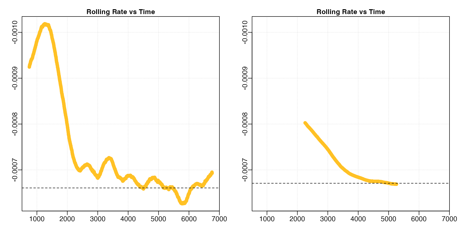

For the linear method, since KDE automatically aggregates stable values, a poor selection of the width may result in a badly-characterised rolling rate estimate output. Under perfectly linear conditions, that is completely monotonic rates, we would expect a rolling regression output plot such as this to consist of a straight, horizontal line. In these data, while the default width allowed a pattern of relative stability in rate after around 2500 seconds to be identified, this information was lost when a width of 0.6 was used, with stable rates only being identified much later in the dataset.

Similarly, if we are interested in highest rate values, under the lower width input we could see values around -0.0010 occurring within the first 1000s of the experiment. This information was also completely lost under the higher width input.

Underfitting

By contrast, if the width is too low the rolling rate is unstable and heavily influenced by data noise and residual variation. This leads to poor results for the linear method, and also highly variable results under the other methods.

Here we’ll compare the default width = 0.2 to a lower value of 5% of the data, width = 0.05.

# Perform linear detection; default width when not specified is 0.2:
normx <- auto_rate(sardine.rd)
#> auto_rate: Applying default 'width' of 0.2

# Perform linear detection using manual width of 0.05:
underx <- auto_rate(sardine.rd, width = 0.05)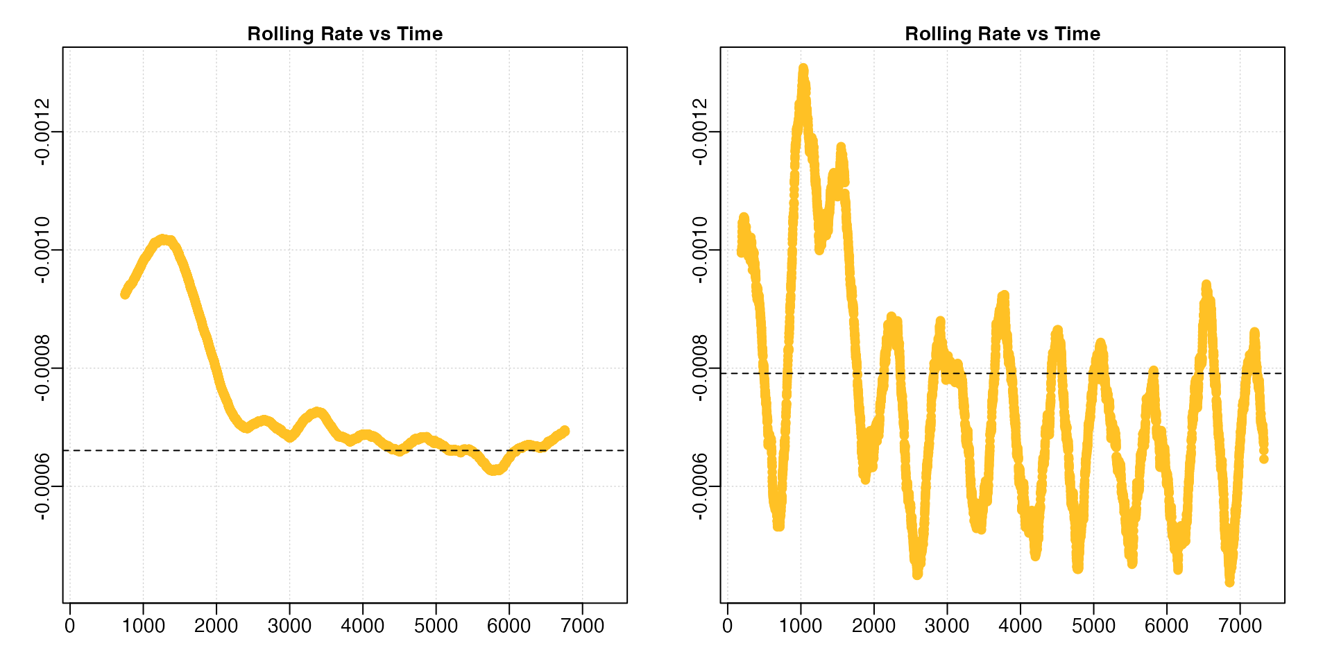

A lower width leads to much more variable rolling rate estimates. Note how we have had to adjust the y-axis limits to fit the results (the left plot is the same data as in the previous section with different axis values). In this particular analysis (results not shown) the linear method performed poorly. If we were interested in highest or lowest rates, this would also prove problematic since the rates are so variable.

Appropriate widths

The width value should be carefully considered; too low and it fails to capture accurate rolling rates and is unduly influenced by data noise or variability, too high and the data is overfitted with important physiological or behavioural states smoothed out. Whatever value is used, this should be reported in the analytical methods alongside results.

See Prinzing et al. 2021 for an excellent discussion of appropriate widths in rolling regressions to determine maximum metabolic rates, much of which is relevant to extracting rates of any kind.

Example Analysis

Here we’ll run through examples of how to use auto_rate to extract rates from respirometry data.

Automatic detection of linear rates

By default, auto_rate identifies the most linear regions of the data (i.e. method = "linear"):

sard_ar <- auto_rate(sardine.rd)
#> auto_rate: Applying default 'width' of 0.2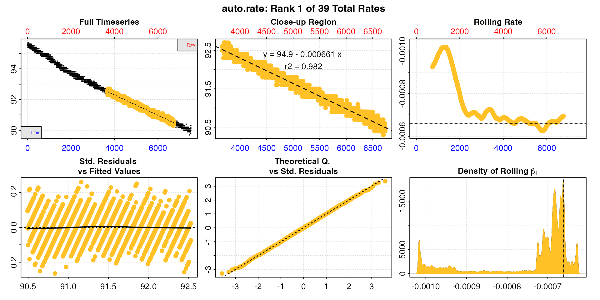

This method detects the most consistently linear regions of the data, that is the most consistent rates observed during the experiment. It does this in a rigorous, unsupervised manner, with the advantage being that this removes observer subjectivity in choosing which rate is most appropriate to report in their results. It is a statistically robust way of indentifying and reporting consistent rates in respirometry data, such as those representative of routine or standard metabolic rates.

Interpreting the plots

The linear method uses the input width as a starting seed value to calculate a rolling rate (panel 3). It then uses these rates to identify linear regions using kernel density estimation (KDE, panel 6). Peaks in this plot represent linear regions, that is areas of stable rates at that width representative of that region as a whole. It then re-samples these regions and runs additional linear analysis at different widths to arrive at a final rate. This is why the final, high ranked rates tend to be over widths greater than the input width, as can be seen here with the top ranked result.

Generally, the higher and wider the peak in the KDE plot, the more linear the region. Here there are several (the current plotted one denoted by a vertical dashed line) and the strongest results are towards the end of the data, including the highest ranked result. The rate value of the current plotted result can also be seen in panel 3 as a horizontal line. This can help assess if it is a representative rate, although bear in mind these rolling rates are at a different width.

See Plot section below for more information.

Exploring the results

Typically, auto_rate will identify multiple linear regions. These are ranked using the kernel density analysis, with the results reflected in the ordering of the $summary table in the output, which is ordered by the $density column. The first row is the top ranked, most linear region, and subsequent rows progressively lower rank. By default, this highest ranked result is returned when print or plot are used, but other results can be output using the pos input with those functions.

print(sard_ar, pos = 2)
#> 
#> # print.auto_rate # ---------------------
#> Data extracted by 'row' using 'width' of 1502.
#> Rates computed using 'linear' method.39 linear regions detected in the kernel density estimate.
#> To see all results use summary().
#> 
#> Position 2 of 39 :
#> Rate: -0.000688 
#> R.sq: 0.986 
#> Rows: 2242 to 5543 
#> Time: 2241 to 5542 
#> -----------------------------------------

plot(sard_ar, pos = 2)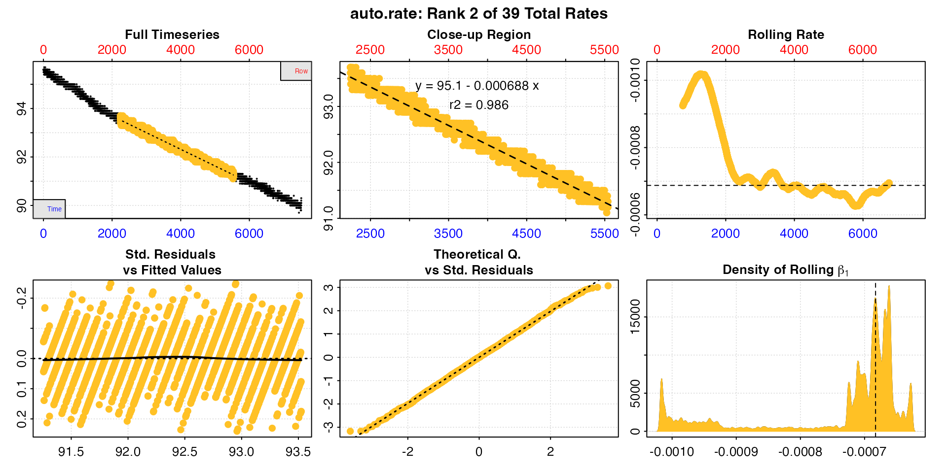

Users should take special note that as an automated, unsupervised machine learning method of identifying linear data auto_rate is fallible, and the results should always be inspected and explored. In this case the function has identified a total of 46 linear regions. They can be viewed by calling summary()

summary(sard_ar)
#> 
#> # summary.auto_rate # -------------------
#> 
#> === Summary of Results by Kernel Density Rank ===
#>     rep rank intercept_b0  slope_b1   rsq density  row endrow time endtime  oxy endoxy      rate
#>  1:  NA    1         94.9 -0.000661 0.982   19069 3659   6736 3658    6735 92.6   90.4 -0.000661
#>  2:  NA    2         95.1 -0.000688 0.986   17461 2242   5543 2241    5542 93.7   91.2 -0.000688
#>  3:  NA    3         94.9 -0.000662 0.987   15969 3628   7164 3627    7163 92.5   90.2 -0.000662
#>  4:  NA    4         95.1 -0.000708 0.979    9204 1578   4236 1577    4235 94.2   92.2 -0.000708
#>  5:  NA    5         95.1 -0.000706 0.971    7555 1947   4236 1946    4235 93.8   92.2 -0.000706
#> ---                                                                                             
#> 35:  NA   35         95.5 -0.000894 0.938     421 1063   2394 1062    2393 94.5   93.5 -0.000894
#> 36:  NA   36         95.5 -0.000894 0.937     388 1066   2393 1065    2392 94.7   93.4 -0.000894
#> 37:  NA   37         95.3 -0.000803 0.929     375 1315   2641 1314    2640 94.3   93.3 -0.000803
#> 38:  NA   38         95.3 -0.000803 0.929     369 1317   2641 1316    2640 94.3   93.3 -0.000803
#> 39:  NA   39         95.3 -0.000803 0.928     322 1325   2635 1324    2634 94.2   93.3 -0.000803
#> 
#> Regressions : 6012 | Results : 39 | Method : linear | Roll width : 1502 | Roll type : row 
#> -----------------------------------------

In this case the first rate result looks good: it has a high r-squared, is sustained over a duration of 50 minutes, and the rate value is consistent with the other results. However in some cases, other ranked results may be more appropriate to report depending on the metabolic rate metric being investigated.

While the first result is the highest in terms of the kernel density value, the user is free to select and report other linear results if they satisfy other desirable criteria, for instance are above a particular r-squared value or span a minimum time window. One peculiarity to take note of in the KDE analysis, is that sometimes the top ranked result does not necessarily have the highest r-squared. This is a counter intuitive result, but explained by the fact that the function learns the shape of the entire dataset, so a particular regression from a linear region might be most representative of the rates in that region, but just happen to be fit to values which return a lower r-squared. This does not mean it is not a valid result; arguably, it is more valid, since it is accurately describing the localised shape of the data. See Chabot et al. (2021) for discussion of r-squared values in metabolic rate measurements.

The pos input can also be used in summary to view particular row ranges. We’ll look at the first 10.

summary(sard_ar, pos = 1:10)
#> 
#> # summary.auto_rate # -------------------
#> 
#> === Summary of results from entered 'pos' rank(s) ===
#> 
#>     rep rank intercept_b0  slope_b1   rsq density  row endrow time endtime  oxy endoxy      rate
#>  1:  NA    1         94.9 -0.000661 0.982   19069 3659   6736 3658    6735 92.6   90.4 -0.000661
#>  2:  NA    2         95.1 -0.000688 0.986   17461 2242   5543 2241    5542 93.7   91.2 -0.000688
#>  3:  NA    3         94.9 -0.000662 0.987   15969 3628   7164 3627    7163 92.5   90.2 -0.000662
#>  4:  NA    4         95.1 -0.000708 0.979    9204 1578   4236 1577    4235 94.2   92.2 -0.000708
#>  5:  NA    5         95.1 -0.000706 0.971    7555 1947   4236 1946    4235 93.8   92.2 -0.000706
#>  6:  NA    6         95.7 -0.001047 0.961    6862  601   1969  600    1968 95.1   93.7 -0.001047
#>  7:  NA    7         95.1 -0.000709 0.978    6395 1578   4196 1577    4195 94.2   92.2 -0.000709
#>  8:  NA    8         94.8 -0.000628 0.929    6285 5050   6613 5049    6612 91.4   90.5 -0.000628
#>  9:  NA    9         94.7 -0.000619 0.912    2609 5123   6507 5122    6506 91.5   90.6 -0.000619
#> 10:  NA   10         95.7 -0.001043 0.961    1917  596   1981  595    1980 95.0   93.6 -0.001043
#> 
#> Regressions : 6012 | Results : 39 | Method : linear | Roll width : 1502 | Roll type : row 
#> -----------------------------------------

Here, the 6th ranked result, while being a valid linear region, is conspicuously higher in rate value and occurs close to the start of the experiment. If we were interested in routine or standard metabolic rates, we would want to exclude this one, as it suggests the specimen might not yet be acclimated to the chamber.

In most cases the best option is to use the top ranked result unless there are specific reasons to exclude it. However, an investigator may opt to select several and take a mean of the resulting rates. For instance here, we might decide on a mean of the top 3 since they have the highest $density values (note that typically we would do this after rates have been adjusted and converted - see later sections - but it is possible here too). We could just average the top 3 values ourselves, but the mean function will also work with auto_rate objects and accepts the pos input.

mean(sard_ar, pos = 1:3)
#> 
#> # mean.auto_rate # ----------------------
#> Mean of rate results from entered 'pos' ranks:
#> 
#> Mean of 3 output rates:
#> [1] -0.00067
#> -----------------------------------------

Any rate value determined after such selection can be saved as a variable, or entered manually as a value in later functions such as adjust_rate and convert_rate. It can also be exported as a value by using export = TRUE in the mean call. However, see next section.

`select_rate`

Alternative selection criteria might also be applied. This might include excluding all results below a certain r-squared, use only the top n’th percentile of results, or exclude those from the certain stages of the experiment.

New in respR v2.0 is the select_rate() function which can apply these criteria, along with many others, to auto_rate results after they have been converted in convert_rate. See vignette("select_rate") for how to do advanced filtering of these results.

Highest rates

auto_rate can also be used to detect the highest and lowest rates over a fixed width. This allows for consistent reporting of respirometry results, such as the highest or lowest rates sustained over a specified time period.

Here we want to know the highest rates sustained over 15 minutes, or 900s, in the sardine.rd data. Since in these data, oxygen is recorded every second and inspect() tells us the time data is gapless and evenly spaced, we can simply specify width in the same number of rows.

sard_insp <- inspect(sardine.rd)
#> inspect: Applying column default of 'time = 1'
#> inspect: Applying column default of 'oxygen = 2'
#> inspect: No issues detected while inspecting data frame.
#> 
#> # print.inspect # -----------------------
#>                 Time Oxygen
#> numeric         pass   pass
#> Inf/-Inf        pass   pass
#> NA/NaN          pass   pass
#> sequential      pass      -
#> duplicated      pass      -
#> evenly-spaced   pass      -
#> 
#> -----------------------------------------

high_rate <- auto_rate(sard_insp, width = 900, by = "row", method = "highest")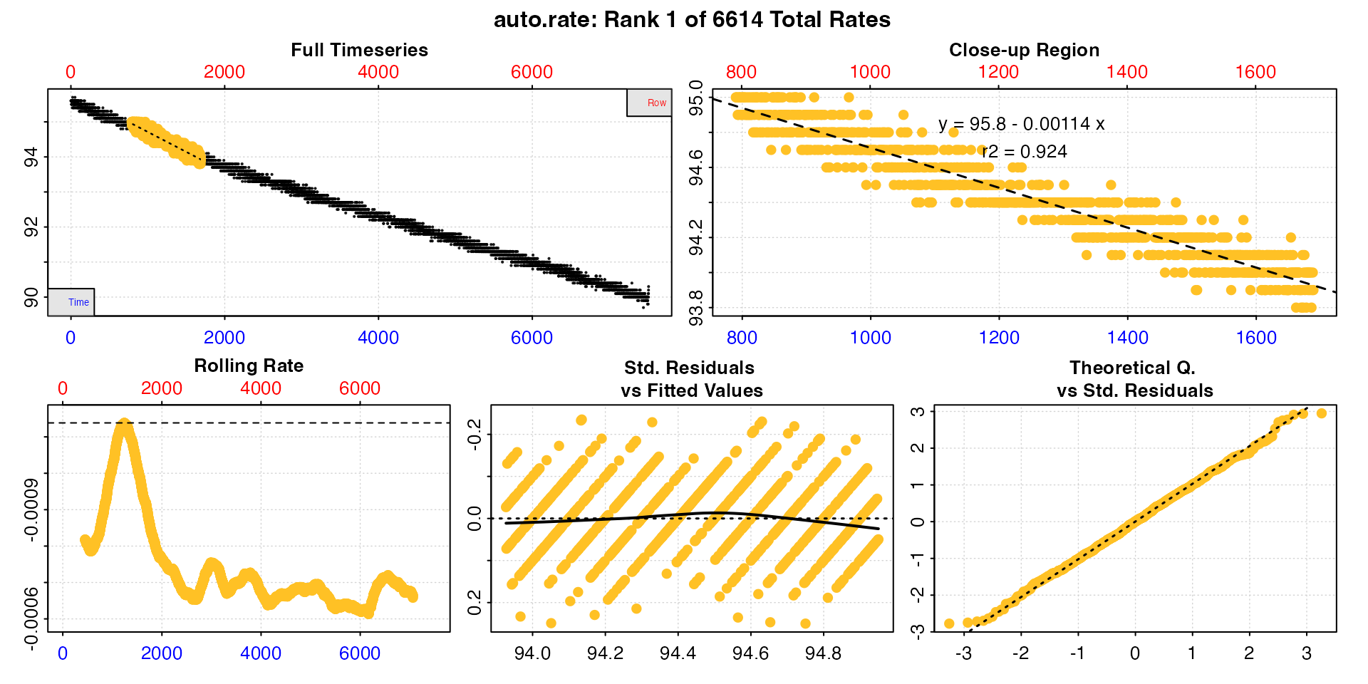

summary(high_rate)
#> 
#> # summary.auto_rate # -------------------
#> 
#> === Summary of Results by Highest Rate ===
#>       rep rank intercept_b0  slope_b1   rsq density  row endrow time endtime  oxy endoxy      rate
#>    1:  NA    1         95.8 -0.001138 0.924      NA  791   1690  790    1689 95.0   93.9 -0.001138
#>    2:  NA    2         95.8 -0.001138 0.924      NA  798   1697  797    1696 95.0   93.8 -0.001138
#>    3:  NA    3         95.8 -0.001138 0.924      NA  792   1691  791    1690 95.0   93.9 -0.001138
#>    4:  NA    4         95.8 -0.001138 0.924      NA  793   1692  792    1691 95.0   93.9 -0.001138
#>    5:  NA    5         95.8 -0.001138 0.924      NA  797   1696  796    1695 95.0   93.8 -0.001138
#>   ---                                                                                             
#> 6610:  NA 6610         94.7 -0.000615 0.793      NA 5717   6616 5716    6615 91.3   90.6 -0.000615
#> 6611:  NA 6611         94.7 -0.000615 0.792      NA 5723   6622 5722    6621 91.1   90.7 -0.000615
#> 6612:  NA 6612         94.7 -0.000615 0.793      NA 5715   6614 5714    6613 91.1   90.5 -0.000615
#> 6613:  NA 6613         94.7 -0.000614 0.792      NA 5720   6619 5719    6618 91.1   90.5 -0.000614
#> 6614:  NA 6614         94.7 -0.000613 0.792      NA 5719   6618 5718    6617 91.2   90.7 -0.000613
#> 
#> Regressions : 6614 | Results : 6614 | Method : highest | Roll width : 900 | Roll type : row 
#> -----------------------------------------

In the highest and lowest methods the rates are ordered by the absolute rate value, regardless of the sign. The top results here have the same rate value as printed, but likely have small differences at higher precision (what you see printed depends on your own R options() settings). Again, a user may choose to report the top result or perform further selection and filtering using select_rate() after conversion in convert_rate. This includes the option to remove rates which overlap, that is share the same rows of data; as we can see here the top results all come from the same region of the data.

Lowest rates

We can similarly find the lowest rate over 15 minutes.

low_rate <- auto_rate(sard_insp, width = 900, method = "lowest")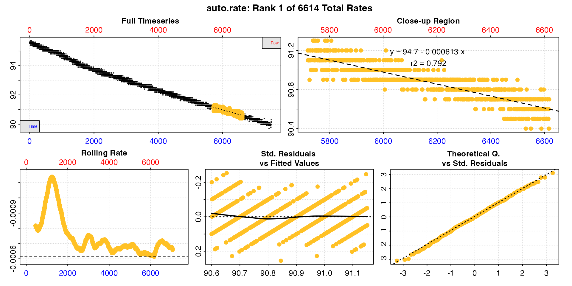

print(low_rate)
#> 
#> # print.auto_rate # ---------------------
#> Data extracted by 'row' using 'width' of 900.
#> Rates computed using 'lowest' method.To see all results use summary().
#> 
#> Position 1 of 6614 :
#> Rate: -0.000613 
#> R.sq: 0.792 
#> Rows: 5719 to 6618 
#> Time: 5718 to 6617 
#> -----------------------------------------

summary(low_rate)
#> 
#> # summary.auto_rate # -------------------
#> 
#> === Summary of Results by Lowest Rate ===
#>       rep rank intercept_b0  slope_b1   rsq density  row endrow time endtime  oxy endoxy      rate
#>    1:  NA    1         94.7 -0.000613 0.792      NA 5719   6618 5718    6617 91.2   90.7 -0.000613
#>    2:  NA    2         94.7 -0.000614 0.792      NA 5720   6619 5719    6618 91.1   90.5 -0.000614
#>    3:  NA    3         94.7 -0.000615 0.793      NA 5715   6614 5714    6613 91.1   90.5 -0.000615
#>    4:  NA    4         94.7 -0.000615 0.792      NA 5723   6622 5722    6621 91.1   90.7 -0.000615
#>    5:  NA    5         94.7 -0.000615 0.793      NA 5717   6616 5716    6615 91.3   90.6 -0.000615
#>   ---                                                                                             
#> 6610:  NA 6610         95.8 -0.001138 0.924      NA  797   1696  796    1695 95.0   93.8 -0.001138
#> 6611:  NA 6611         95.8 -0.001138 0.924      NA  793   1692  792    1691 95.0   93.9 -0.001138
#> 6612:  NA 6612         95.8 -0.001138 0.924      NA  792   1691  791    1690 95.0   93.9 -0.001138
#> 6613:  NA 6613         95.8 -0.001138 0.924      NA  798   1697  797    1696 95.0   93.8 -0.001138
#> 6614:  NA 6614         95.8 -0.001138 0.924      NA  791   1690  790    1689 95.0   93.9 -0.001138
#> 
#> Regressions : 6614 | Results : 6614 | Method : lowest | Roll width : 900 | Roll type : row 
#> -----------------------------------------

Note, the output objects of the highest and lowest methods are essentially identical, the only difference being the results are ordered descending or ascending by absolute rate value.

Rolling rates

The rolling method allows a rolling regression of the specified width to be returned in sequential order.

roll_rate <- auto_rate(sard_insp, width = 900, method = "rolling")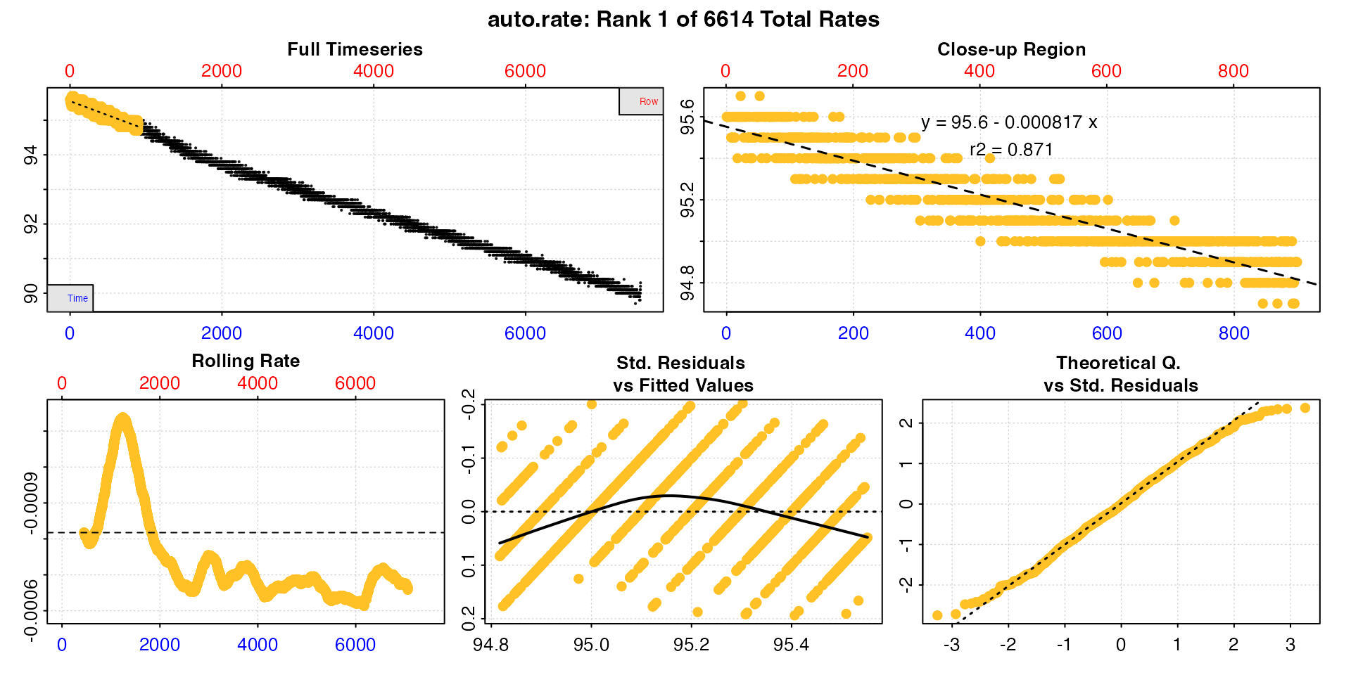

summary(roll_rate)
#> 
#> # summary.auto_rate # -------------------
#> 
#> === Summary of Results by Rolling Order ===
#>       rep rank intercept_b0  slope_b1   rsq density  row endrow time endtime  oxy endoxy      rate
#>    1:  NA    1         95.6 -0.000817 0.871      NA    1    900    0     899 95.6   94.9 -0.000817
#>    2:  NA    2         95.6 -0.000818 0.871      NA    2    901    1     900 95.6   94.7 -0.000818
#>    3:  NA    3         95.6 -0.000817 0.871      NA    3    902    2     901 95.6   94.9 -0.000817
#>    4:  NA    4         95.6 -0.000817 0.871      NA    4    903    3     902 95.6   94.7 -0.000817
#>    5:  NA    5         95.6 -0.000817 0.871      NA    5    904    4     903 95.6   94.8 -0.000817
#>   ---                                                                                             
#> 6610:  NA 6610         95.0 -0.000666 0.845      NA 6610   7509 6609    7508 90.6   90.0 -0.000666
#> 6611:  NA 6611         95.0 -0.000665 0.844      NA 6611   7510 6610    7509 90.7   90.1 -0.000665
#> 6612:  NA 6612         94.9 -0.000663 0.843      NA 6612   7511 6611    7510 90.7   90.1 -0.000663
#> 6613:  NA 6613         94.9 -0.000660 0.841      NA 6613   7512 6612    7511 90.5   90.2 -0.000660
#> 6614:  NA 6614         94.9 -0.000658 0.837      NA 6614   7513 6613    7512 90.5   90.3 -0.000658
#> 
#> Regressions : 6614 | Results : 6614 | Method : rolling | Roll width : 900 | Roll type : row 
#> -----------------------------------------

This outputs every regression of the width in order. The main utility of this method is for passing to select_rate after conversion in convert_rate where various criteria can be applied to filter the results manually. See vignette("select_rate").

Further processing

Saved auto_rate objects can be passed to subsequent respR functions for further processing, such as adjust_rate() to adjust for background respiration, or convert_rate() to convert to final oxygen uptake units. See other vignettes for examples of these operations.

Plot

When using auto_rate, a plot of the results is produced (unless plot = FALSE). If there are multiple results each can be plotted individually using pos. Each panel can be plotted on its own using panel with values 1 to 6. If labels or legends obscure parts of the plot they can be suppressed using legend = FALSE. Console output messages can be suppressed with quiet = TRUE. Lastly, the rolling rate plot can be plotted on an unreversed y-axis with rate.rev = FALSE, if for instance you are examining oxygen production rates.

The first panel is the complete timeseries of oxygen against both time (bottom blue axis) and row index (top red axis) with the pos rate regression (defualt is pos = 1) highlighted in yellow. The next plot is a close-up of this rate region. The next is a rolling rate plot across the entire timeseries at the input width (see here). The next two are diagnostic plots of the fitted values vs. residuals for the current rate result. Lastly, the sixth panel (only for the linear method) is a plot of the kernel density analysis output, which is the density peaks of stable rate values.

See Interpreting the plots section above for more information.

Notes

auto_rate does not currently support analysis of flowthrough respirometry data. See vignette("flowthrough") for analysis of these experiments.
The auto_rate linear method works best with data that is fairly monotonic, that is shows an either downward or upward trend without strong fluctuations. With intermittent-flow respirometry data there is a strong possibility flush periods will confuse the auto_rate algorithms, so it should typically only be run on subsets of the data containing actual specimen measurements. The subset_data function is ideal for subsetting and passing data regions of interest to other functions. See vignette("intermittent_long").

Introduction

Overview

Rolling linear regression

Methods

method = "linear"

When this method might be applied

method = "lowest"

When this method might be applied

method = "highest"

When this method might be applied

method = "minimum", method = "maximum"

When these methods might be applied

method = "rolling"

When this method might be applied

method = "interval"

When this method might be applied

Adjusting the width

Overfitting

Underfitting

Appropriate widths

Example Analysis

Automatic detection of linear rates

Interpreting the plots

Exploring the results

select_rate

Highest rates

Lowest rates

Rolling rates

Further processing

Plot

Notes

`method = "linear"`

`method = "lowest"`

`method = "highest"`

`method = "minimum"`, `method = "maximum"`

`method = "rolling"`

`method = "interval"`

`select_rate`