Identifies critical oxygen values, the oxygen tension or concentration below which an uptake rate transitions from independent to dependent on the oxygen supply, typically known as PCrit.
Usage
oxy_crit(
  x,
  method = "bsr",
  time = NULL,
  oxygen = NULL,
  rate = NULL,
  width = 0.1,
  parallel = FALSE,
  thin = 5000,
  plot = TRUE,
  ...
)
Arguments
- x
object of class
inspector adata.framecontaining either paired oxygen~time values, or paired rate~oxygen values. See Details.- method
string. Defaults to
"bsr". Critical oxygen value analysis method. Either"bsr"or"segmented". See Details.- time
integer or string. Defaults to 1. Specifies column number or column name of the time data.
- oxygen
integer or string. Defaults to 2. Specifies column number or column name of the oxygen data.
- rate
integer or string. Defaults to NULL. Specifies column number or column name of the rate data.
- width
numeric value between 0 and 1 representing proportion of the total data length. Determines the width of the rolling regression used to determine the rolling rate and the rolling mean of oxygen values the rate is paired with. Defaults to 0.1, representing 10% of total rows.
- parallel
logical. Defaults to FALSE. Enables parallel processing for computationally intensive analyses of large datasets.
- thin
integer. Defaults to 5000. Number of rows to subsample
xdata to before running"bsr"analysis. No effect on datasets smaller than this value or with"segmented"method. To perform no subsampling enter asNULL. See Details.- plot
logical. Defaults to TRUE.
- ...
Allows additional plotting controls to be passed, such as
legend = FALSE,quiet = TRUE,rate.rev = FALSE, andpanel. See Plotting section.
Value
Output is a list object of class oxy_crit containing input
parameters and data, various summary data, metadata, and the primary output
of interest $crit, which is the critical oxygen value in the units of the
oxygen data as entered. This can be converted to additional units using
convert_DO(). Note, if the Broken-Stick analysis (method == "bsr")
has been used, $crit will contain two results; $crit.intercept and
$crit.midpoint. For full explanation of the difference between these see
Yeager & Ultsch (1989), however they are generally very close in value.
Details
In earlier versions of respR, this function was known as pcrit or
calc_pcrit. It was renamed to avoid conflicts with functions of the same
name in another package, and also because technically the P in PCrit
stands for the partial pressure of oxygen. Since the function returns the
value in the units of the data as entered, whether they are concentration or
pressure units, this terminology can be technically in error. Instead, for
the purposes of the documentation we refer to this as the Critical Oxygen
Value, or "COV". If the units of oxygen are partial pressure units (e.g.
kPa), this is equivalent to PCrit, otherwise they should be reported with
this in mind.
Methods
The oxy_crit() function provides two methods (one of which outputs two
results) to calculate the COV. These are selected using the method input.
Broken Stick Regression: method = "bsr"
This is the default method, adapted from the “Broken-Stick” regression (BSR) approach, of Yeager & Ultsch (1989), in which two segments of the data are iteratively fitted and the intersection with the smallest sum of the residual sum of squares between the two linear models is the estimated COV. Two slightly different ways of reporting this breakpoint are detailed by Yeager & Ultsch (1989); the intercept and midpoint. These are usually very close in value, and the function returns both.
The thin input influences the BSR analysis. The method is very
computationally intensive, so to speed up analyses the thin input will
subsample datasets longer than this input to this number or rows before
analysis. The default value of 5000 has in testing provided a good balance
between speed and results accuracy and repeatability. However, results may
vary with different datasets, so users should experiment with varying the
value. To perform no subsampling and use the entire dataset enter thin = NULL. It has no effect on datasets shorter than the thin input.
Segmented Regression: method = "segmented"
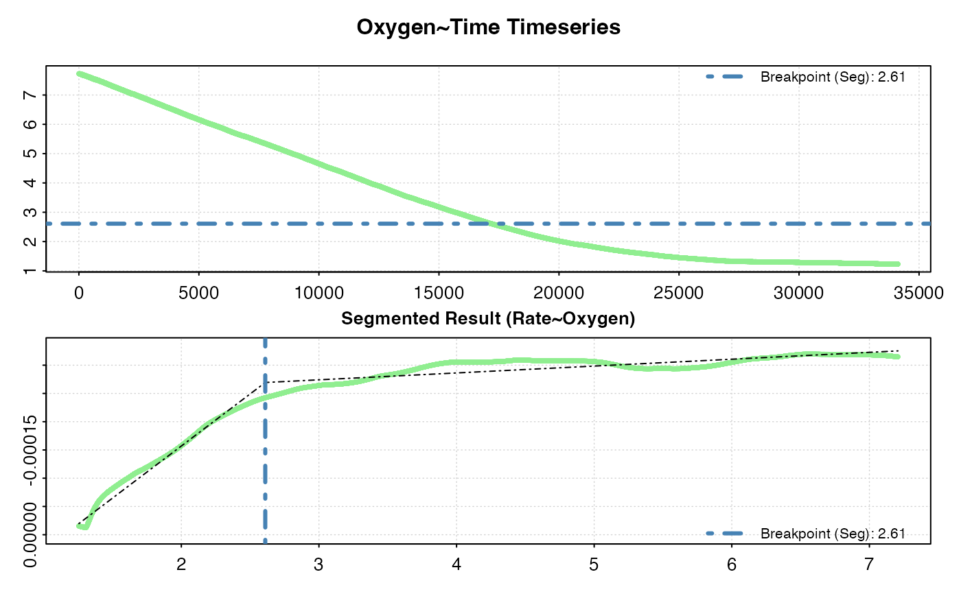
The second method is a wrapper for the "Segmented" regression approach,
available as part of the segmented R package (Muggeo 2008), which estimates
the COV by iteratively fitting two intersecting models and selecting the
value that minimises the “gap” between the fitted lines.
Inputs
The data input x should be an inspect object or data.frame containing
oxygen~time data, or a data.frame containing rate~oxygen data.
Oxygen ~ Time data
This is the typical input, where a timeseries of oxygen concentrations or
partial pressures against time has been recorded, generally down to a very
low value of oxygen. A column of time and a column of oxygen should be
specified. The function defaults to time = 1 and oxygen = 2 if no other
inputs are entered. These can also be specified using the column names.
If an inspect object is entered as the x input, the data frame is
extracted automatically and column identifiers are not required since these
were already entered in inspect. Note, if multiple oxygen columns were
entered in inspect only the first entered one will be used in oxy_crit.
To calculate the COV, the function requires data in the form of oxygen
uptake rate against oxygen value. Therefore, the function performs a rolling
regression on the oxygen~time data to determine rates, and pairs these
against a rolling mean of the oxygen data. The function then performs the
selected analysis method on these data. The width of the rolling regression
and rolling mean is determined by the width input. The default is 0.1,
representing 10% of the length of the data. This performs well in testing,
however performance may vary with data that has abrupt changes in rate, or is
particularly noisy. Users should experiment with different width values to
see how it affects results, and report this with their results and analysis
parameters.
Rate ~ Oxygen data
Alternatively, if existing rolling oxygen uptake rates have been calculated,
and have appropriate paired oxygen concentration or partial pressure values,
these can be entered with the rate and oxygen inputs specifying the
respective columns as either numbers or the column names. In this case the
function performs the selected analysis method on these data directly
without any processing. The width input in this case is not relevant and is
ignored.
This option can only be used with data frame x inputs. Note, other columns
such as time data may be present in the input, but are not required so need
not be specified.
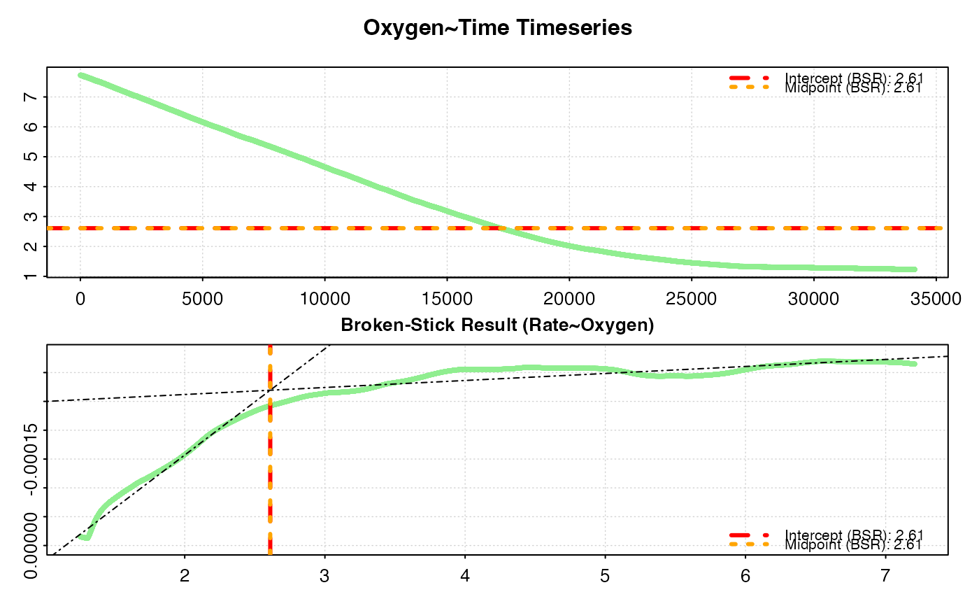
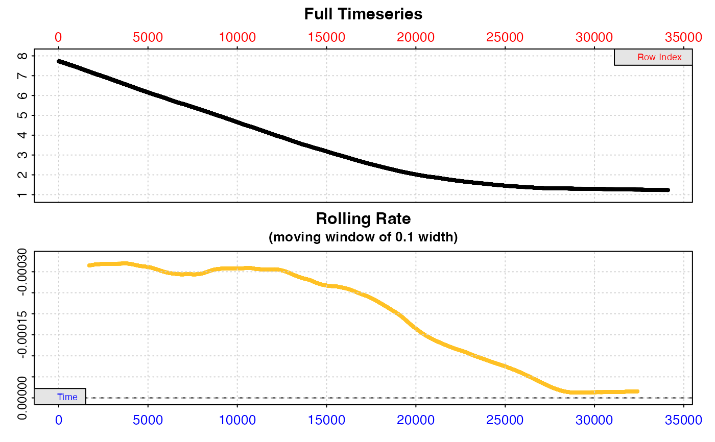
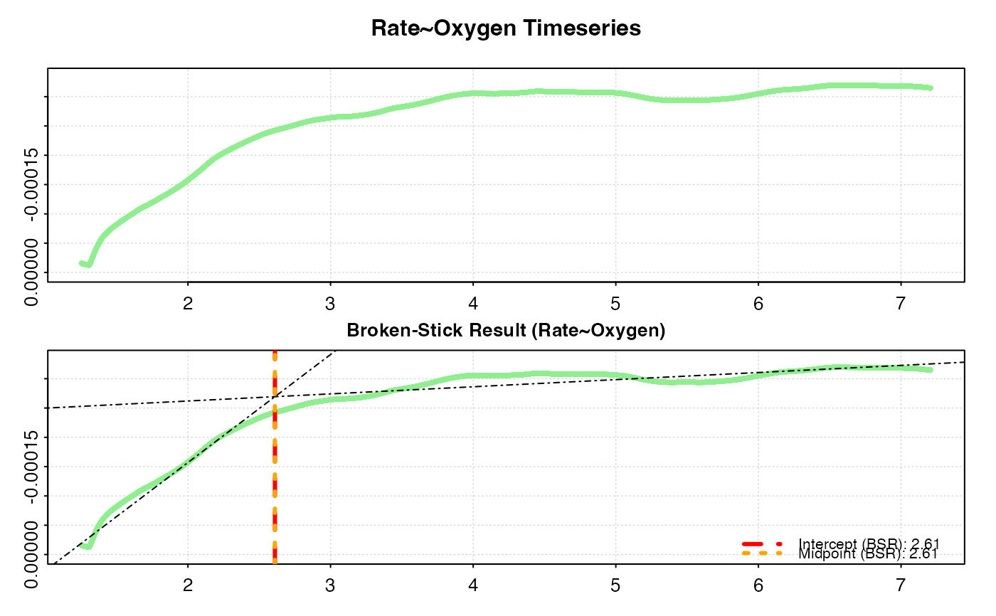
Plot
A plot is produced (provided plot = TRUE) of the input data and results.
The top panel is the input data, either the oxygen~time timeseries, or the
rate~oxygen series, depending on what was entered in x. If the former, the
critical oxygen value is indicated by a horizontal line, or two lines in the
case of the Broken-Stick analysis. Note, since the two BSR results are
usually close in value these may overlay each other.
The bottom plot is the rate~oxygen series upon which the analysis was conducted, either as input or as calculated. Critical oxygen values are indicated by vertical lines, and regression fits upon which the analysis was based by black dashed lines.
Note, that in respR oxygen uptake rates are negative since they represent a
negative slope of oxygen against time, therefore by default rates are plotted
on a reverse y-axis so higher rates appear higher on the plot. If analysing
already calculated rates which are positive values this behaviour can be
reversed by passing rate.rev = FALSE in either the main function call or
when calling plot() on the output object. There is no issue with using
positive rate values; they will give identical critical value results in the
analysis.
Additional plotting options
If the legend obscures parts of the plot they can be suppressed using legend = FALSE. Suppress console output messages with quiet = TRUE. Each panel
can be plotted on its own using panel = 1 or panel = 2. If using
already-calculated, positive rate values to identify critical oxygen values,
the y-axis of the rolling rate plot can be plotted not reversed by passing
rate.rev = FALSE These inputs can be passed in either the main oxy_crit
call or when calling plot() on the output object. If axis labels
(particularly y-axis) are difficult to read, las = 2 can be passed to make
axis labels horizontal, and oma (outer margins, default oma = c(0.4, 1, 1.5, 0.4)), and mai (inner margins, default mai = c(0.3, 0.15, 0.35, 0.15)) used to adjust plot margins.
S3 Generic Functions
Saved output objects can be used in the generic S3 functions print() and
summary().
print(): prints the critical oxygen value for the particularmethodused.summary(): prints critical oxygen value, plus additional coefficients and metadata for the particularmethodused. See Yeager & Ultsch (1989) and Muggeo (2008) for what these represent. The summary can be exported as a separate data frame by passingexport = TRUE.
More
For additional help, documentation, vignettes, and more visit the respR
website at https://januarharianto.github.io/respR/
References
Yeager DP, Ultsch GR (1989) Physiological regulation and conformation: A BASIC program for the determination of critical points. Physiological Zoology 62:888–907. doi: 10.1086/physzool.62.4.30157935
Muggeo V (2008) Segmented: an R package to fit regression models with broken-line relationships. R News 8:20–25.
Examples
# \donttest{
## Run on oxygen~time data.frame with default inputs
oxy_crit(squid.rd)
#> oxy_crit: Applying column defaults of 'time = 1' and 'oxygen = 2'.
#> oxy_crit: Performing Broken-Stick analysis (Yeager and Ultsch 1989)...
#> oxy_crit: Broken-Stick analysis completed in 4.6 seconds.
#> plot.oxy_crit: Plotting Oxygen ~ Time derived critical oxygen results.
 #>
#> # print.oxy_crit # ----------------------
#>
#> Broken-Stick (Yeager & Ultsch 1989):
#>
#> Sum RSS 0.0000006404122
#> Intercept 2.610095
#> Midpoint 2.609737
#>
#> -----------------------------------------
## Try a lower 'thin' input to speed up analysis
oxy_crit(squid.rd, thin = 1000)
#> oxy_crit: Applying column defaults of 'time = 1' and 'oxygen = 2'.
#> oxy_crit: Performing Broken-Stick analysis (Yeager and Ultsch 1989)...
#> oxy_crit: Broken-Stick analysis completed in 0.8 seconds.
#> plot.oxy_crit: Plotting Oxygen ~ Time derived critical oxygen results.
#>
#> # print.oxy_crit # ----------------------
#>
#> Broken-Stick (Yeager & Ultsch 1989):
#>
#> Sum RSS 0.0000006404122
#> Intercept 2.610095
#> Midpoint 2.609737
#>
#> -----------------------------------------
## Try a lower 'thin' input to speed up analysis
oxy_crit(squid.rd, thin = 1000)
#> oxy_crit: Applying column defaults of 'time = 1' and 'oxygen = 2'.
#> oxy_crit: Performing Broken-Stick analysis (Yeager and Ultsch 1989)...
#> oxy_crit: Broken-Stick analysis completed in 0.8 seconds.
#> plot.oxy_crit: Plotting Oxygen ~ Time derived critical oxygen results.
 #>
#> # print.oxy_crit # ----------------------
#>
#> Broken-Stick (Yeager & Ultsch 1989):
#>
#> Sum RSS 0.0000001280328
#> Intercept 2.612272
#> Midpoint 2.614072
#>
#> -----------------------------------------
## Use the Segmented method instead
oxy_crit(squid.rd, method = "segmented")
#> oxy_crit: Applying column defaults of 'time = 1' and 'oxygen = 2'.
#> oxy_crit: Performing Segmented breakpoint analysis (Muggeo 2003)...
#> oxy_crit: Segmented analysis convergence attained in 1 iterations.
#> plot.oxy_crit: Plotting Oxygen ~ Time derived critical oxygen results.
#>
#> # print.oxy_crit # ----------------------
#>
#> Broken-Stick (Yeager & Ultsch 1989):
#>
#> Sum RSS 0.0000001280328
#> Intercept 2.612272
#> Midpoint 2.614072
#>
#> -----------------------------------------
## Use the Segmented method instead
oxy_crit(squid.rd, method = "segmented")
#> oxy_crit: Applying column defaults of 'time = 1' and 'oxygen = 2'.
#> oxy_crit: Performing Segmented breakpoint analysis (Muggeo 2003)...
#> oxy_crit: Segmented analysis convergence attained in 1 iterations.
#> plot.oxy_crit: Plotting Oxygen ~ Time derived critical oxygen results.
 #>
#> # print.oxy_crit # ----------------------
#>
#> Segmented (Muggeo 2003):
#>
#> Std. Err. 0.001785221
#> Breakpoint 2.609903
#>
#> -----------------------------------------
## Experiment with different 'width' input
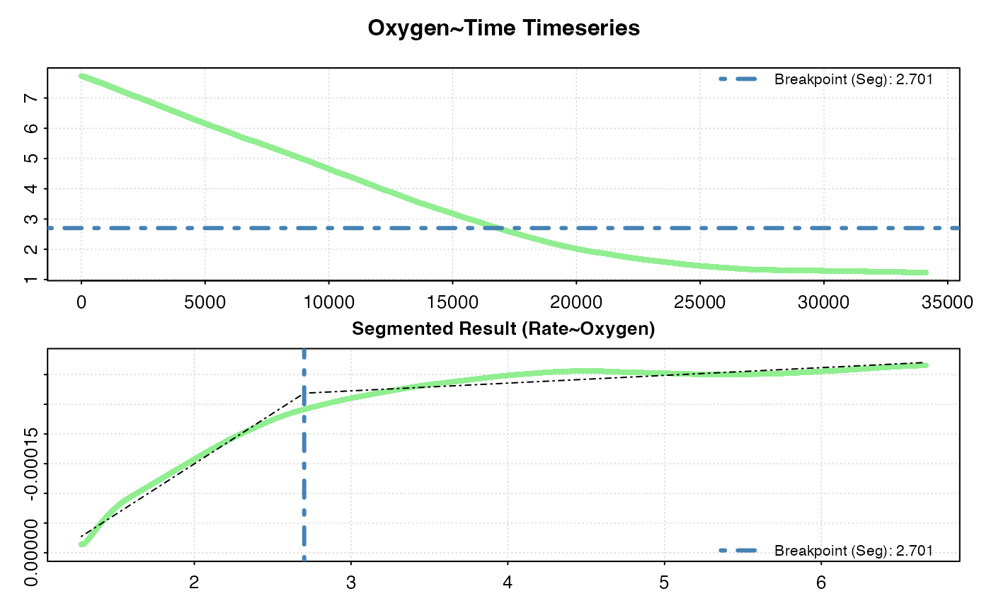
# Higher widths tend to oversmooth data
oxy_crit(squid.rd, method = "segmented", width = 0.2)
#> oxy_crit: Applying column defaults of 'time = 1' and 'oxygen = 2'.
#> oxy_crit: Performing Segmented breakpoint analysis (Muggeo 2003)...
#> oxy_crit: Segmented analysis convergence attained in 1 iterations.
#> plot.oxy_crit: Plotting Oxygen ~ Time derived critical oxygen results.
#>
#> # print.oxy_crit # ----------------------
#>
#> Segmented (Muggeo 2003):
#>
#> Std. Err. 0.001785221
#> Breakpoint 2.609903
#>
#> -----------------------------------------
## Experiment with different 'width' input
# Higher widths tend to oversmooth data
oxy_crit(squid.rd, method = "segmented", width = 0.2)
#> oxy_crit: Applying column defaults of 'time = 1' and 'oxygen = 2'.
#> oxy_crit: Performing Segmented breakpoint analysis (Muggeo 2003)...
#> oxy_crit: Segmented analysis convergence attained in 1 iterations.
#> plot.oxy_crit: Plotting Oxygen ~ Time derived critical oxygen results.
 #>
#> # print.oxy_crit # ----------------------
#>
#> Segmented (Muggeo 2003):
#>
#> Std. Err. 0.00182839
#> Breakpoint 2.701036
#>
#> -----------------------------------------
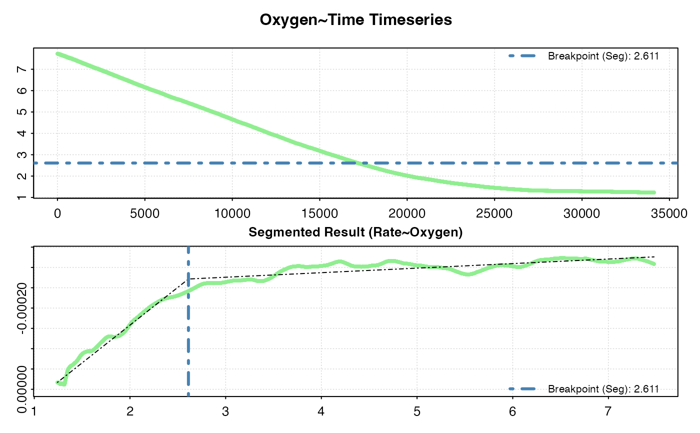
# Lower width in this case gives very similar result to default 0.1
oxy_crit(squid.rd, method = "segmented", width = 0.05)
#> oxy_crit: Applying column defaults of 'time = 1' and 'oxygen = 2'.
#> oxy_crit: Performing Segmented breakpoint analysis (Muggeo 2003)...
#> oxy_crit: Segmented analysis convergence attained in 1 iterations.
#> plot.oxy_crit: Plotting Oxygen ~ Time derived critical oxygen results.
#>
#> # print.oxy_crit # ----------------------
#>
#> Segmented (Muggeo 2003):
#>
#> Std. Err. 0.00182839
#> Breakpoint 2.701036
#>
#> -----------------------------------------
# Lower width in this case gives very similar result to default 0.1
oxy_crit(squid.rd, method = "segmented", width = 0.05)
#> oxy_crit: Applying column defaults of 'time = 1' and 'oxygen = 2'.
#> oxy_crit: Performing Segmented breakpoint analysis (Muggeo 2003)...
#> oxy_crit: Segmented analysis convergence attained in 1 iterations.
#> plot.oxy_crit: Plotting Oxygen ~ Time derived critical oxygen results.
 #>
#> # print.oxy_crit # ----------------------
#>
#> Segmented (Muggeo 2003):
#>
#> Std. Err. 0.001905877
#> Breakpoint 2.611025
#>
#> -----------------------------------------
## Run on oxygen~time data in 'inspect' object
insp <- inspect(squid.rd, time = 1, oxygen = 2)
#> inspect: No issues detected while inspecting data frame.
#>
#> # print.inspect # -----------------------
#> Time Oxygen
#> numeric pass pass
#> Inf/-Inf pass pass
#> NA/NaN pass pass
#> sequential pass -
#> duplicated pass -
#> evenly-spaced pass -
#>
#> -----------------------------------------
#>
#> # print.oxy_crit # ----------------------
#>
#> Segmented (Muggeo 2003):
#>
#> Std. Err. 0.001905877
#> Breakpoint 2.611025
#>
#> -----------------------------------------
## Run on oxygen~time data in 'inspect' object
insp <- inspect(squid.rd, time = 1, oxygen = 2)
#> inspect: No issues detected while inspecting data frame.
#>
#> # print.inspect # -----------------------
#> Time Oxygen
#> numeric pass pass
#> Inf/-Inf pass pass
#> NA/NaN pass pass
#> sequential pass -
#> duplicated pass -
#> evenly-spaced pass -
#>
#> -----------------------------------------
 oxy_crit(insp)
#> oxy_crit: Applying column defaults of 'time = 1' and 'oxygen = 2'.
#> oxy_crit: Performing Broken-Stick analysis (Yeager and Ultsch 1989)...
#> oxy_crit: Broken-Stick analysis completed in 5.4 seconds.
#> plot.oxy_crit: Plotting Oxygen ~ Time derived critical oxygen results.
 #>
#> # print.oxy_crit # ----------------------
#>
#> Broken-Stick (Yeager & Ultsch 1989):
#>
#> Sum RSS 0.0000006404122
#> Intercept 2.610095
#> Midpoint 2.609737
#>
#> -----------------------------------------
## Run on already calculated rate~oxygen data
# Calculate a rolling rate
rate <- auto_rate(squid.rd,
method = "rolling",
width = 0.1,
plot = FALSE)$rate
## Calculate a rolling mean oxygen
oxy <- na.omit(roll::roll_mean(squid.rd[[2]],
width = 0.1 * nrow(squid.rd)))
## Combine to data.frame
squid_rate_oxy <- data.frame(oxy, rate)
## Perform COV analysis
oxy_crit(squid_rate_oxy, oxygen = 1, rate = 2)
#> oxy_crit: Performing analysis using Rate ~ Oxygen data.
#> oxy_crit: Performing Broken-Stick analysis (Yeager and Ultsch 1989)...
#> oxy_crit: Broken-Stick analysis completed in 3.9 seconds.
#> plot.oxy_crit: Plotting Rate ~ Oxygen derived critical oxygen results.
#>
#> # print.oxy_crit # ----------------------
#>
#> Broken-Stick (Yeager & Ultsch 1989):
#>
#> Sum RSS 0.0000006404122
#> Intercept 2.610095
#> Midpoint 2.609737
#>
#> -----------------------------------------
## Run on already calculated rate~oxygen data
# Calculate a rolling rate
rate <- auto_rate(squid.rd,
method = "rolling",
width = 0.1,
plot = FALSE)$rate
## Calculate a rolling mean oxygen
oxy <- na.omit(roll::roll_mean(squid.rd[[2]],
width = 0.1 * nrow(squid.rd)))
## Combine to data.frame
squid_rate_oxy <- data.frame(oxy, rate)
## Perform COV analysis
oxy_crit(squid_rate_oxy, oxygen = 1, rate = 2)
#> oxy_crit: Performing analysis using Rate ~ Oxygen data.
#> oxy_crit: Performing Broken-Stick analysis (Yeager and Ultsch 1989)...
#> oxy_crit: Broken-Stick analysis completed in 3.9 seconds.
#> plot.oxy_crit: Plotting Rate ~ Oxygen derived critical oxygen results.
 #>
#> # print.oxy_crit # ----------------------
#>
#> Broken-Stick (Yeager & Ultsch 1989):
#>
#> Sum RSS 0.0000006404122
#> Intercept 2.610095
#> Midpoint 2.609737
#>
#> -----------------------------------------
# }
#>
#> # print.oxy_crit # ----------------------
#>
#> Broken-Stick (Yeager & Ultsch 1989):
#>
#> Sum RSS 0.0000006404122
#> Intercept 2.610095
#> Midpoint 2.609737
#>
#> -----------------------------------------
# }
